CED: Continuing Context with a Causal Encoder and Decoder

In YOCO, the early layers produced shared KV for the later layers to read. This meant the later layers did not need to compute every past position to produce the first output. With this separation of roles in mind, we can now examine the Causal Encoder–Decoder (CED).

This article covers CED in the DeepSeek-V4.1-Flash report. We will focus on how it uses global information produced by the encoder together with local information produced by the decoder itself. We first trace token generation and the sources of KV, then separate position selection from the attention computation and examine what layers reuse. Finally, we explain the prefill work that remains because the decoder has its own local state.

Comparing Generation Paths with a Traditional Encoder–Decoder

The names encoder and decoder alone do not determine the path of a new token. The left side of Figure 1 shows a T5-style architecture with separate input and output sequences. The right side shows CED, where the prompt and generated tokens form a single sequence.

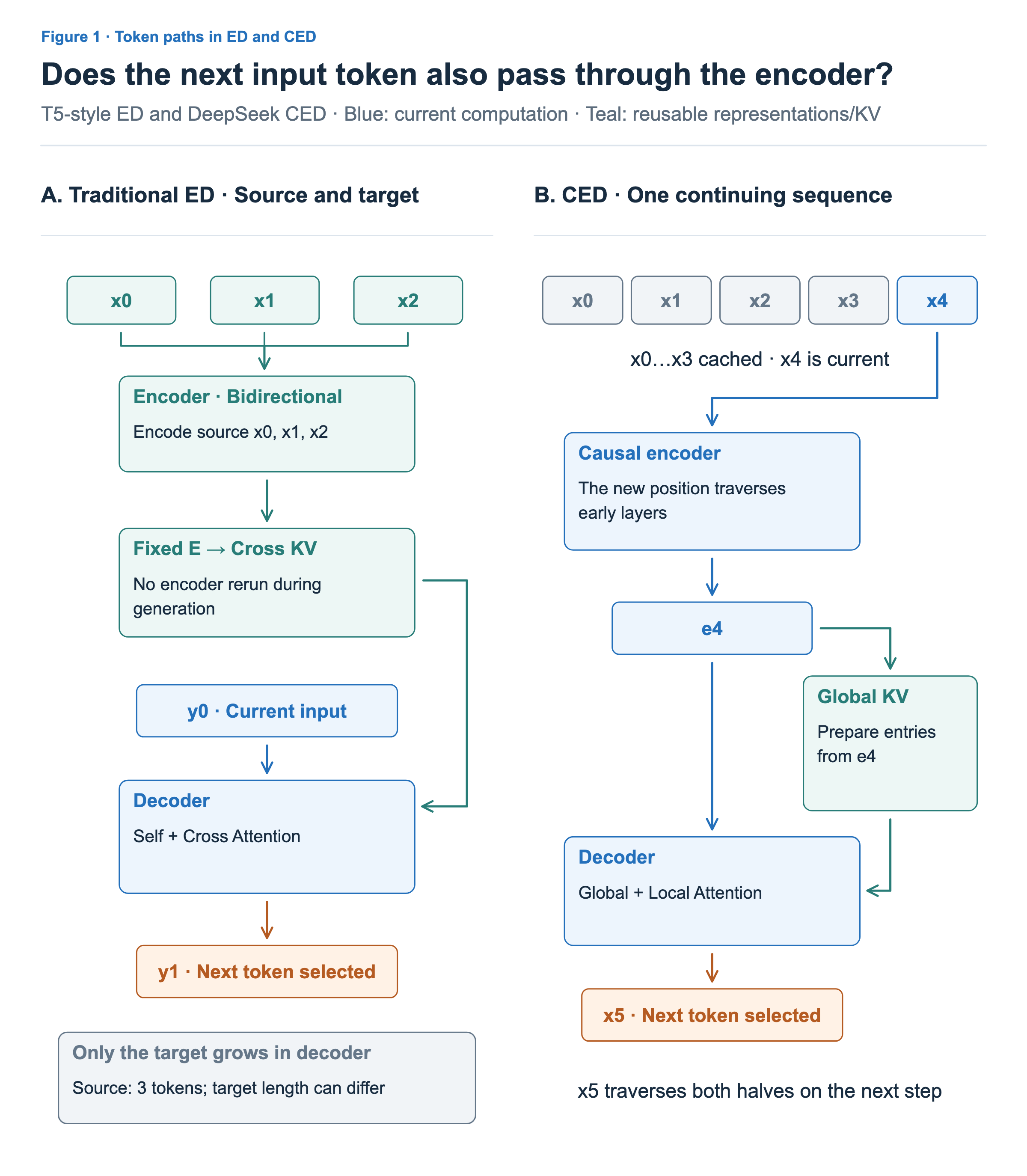
The encoder in a T5-style encoder–decoder processes the entire source bidirectionally. For example, the representation of the first source token can use information from the last source token. The resulting source representations remain available throughout target generation.

The decoder has two reading paths. Causal self-attention reads earlier target positions, while cross-attention reads source information produced by the encoder. Once a selected target token becomes the next input, it passes through the decoder. Generating each token does not inherently require the same source to pass through the encoder again.

In CED, generated tokens follow the prompt. When a new token becomes the next input, it passes through the causal encoder, whose output then enters the decoder. The context produced by the encoder therefore grows as generation proceeds. This explains why the return arrows in the figure lead to different places.

In both cases, selecting a token and processing that token as the next input happen at different times. Immediately after selection, only the new token ID has been determined. Its corresponding state is created during the next execution as it passes through the required layers. The start marker and the one-position shift in the target labels illustrate this prediction order.

One Token Sequence and Causal Access

Let us replace the arrows with position grids. In Figure 2, rows are Query positions and columns are Key positions available for reference. The upper grids show relationships inside the encoder; the lower grids show how the decoder reads encoder information.

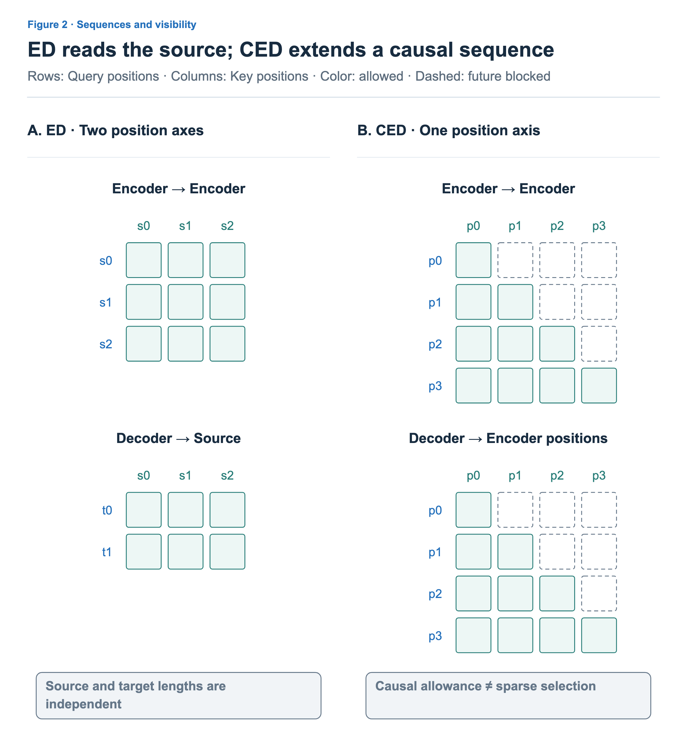
The example on the left has three source positions and two target positions. Source and target lengths are independent, and positions with the same number need not represent corresponding words. Each target Query can read the entire source prepared by the encoder. This is different from reading target answers that have not yet been generated.

On the right, the encoder and decoder process the same token sequence. Encoder information used at p2 must be produced from inputs through p2. Feeding information from p3 into p2 would leak the future into next-token prediction. This produces a triangle that allows the current and earlier positions while blocking future positions.

This figure shows the original position relationships allowed by causality. It is not the list of entries actually selected by sparse attention. A position inside the triangle is safe to read causally; that does not mean every such position is read.

Shared Global KV and Per-Layer Local KV

Figure 3 separates shared storage from per-layer computation in the actual decoder. The left side prepares values that multiple layers read together; the right side shows the work performed anew in each layer.

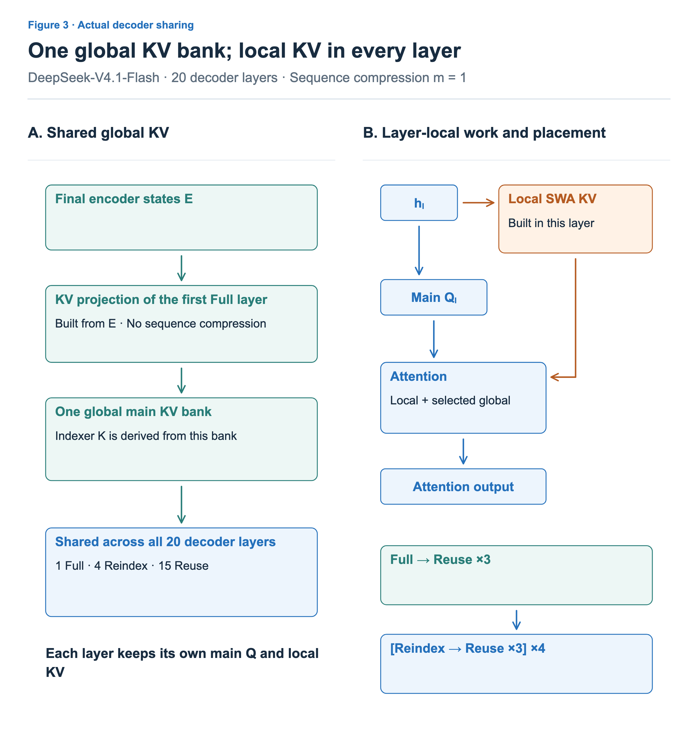
Global KV in CED is projected from the encoder’s final hidden state E. Local KV comes from each decoder layer’s own hidden state. This lets the decoder read both the long context processed by the encoder and the recent context processed at each decoder depth.

Receiving the same E as input is different from sharing the already projected KV values. Different transformations of the same input can produce different results. The general CED formulation allows per-layer projections, but in the actual arrangement shown in Figure 3, all remaining decoder layers share the global KV produced by the first decoder layer. We will examine the reuse modes later.

In contrast, Main Q and Local KV on the right are produced anew in every layer. Here, h is the hidden state entering the current layer, not the original input embedding. Even the same token has a different representation after passing through earlier layers. Each layer therefore produces a different Query for reading shared KV and different Local KV to retain for recent positions.

For example, producing the second decoder layer’s local KV requires representations that have passed through the first layer. Having E ready does not mean the second layer’s local KV is ready. This distinction matters when we determine the scope of prefill computation in the final section.

What Does the Sequence Compression Rate Reduce?

The sequence compression rate m in Figure 3 describes how much the number of global main KV entries is reduced relative to the original number of token positions. With m=2 in CSA2, information from two positions is combined into one entry. In a teaching example containing only complete groups, 8 positions become 8 ÷ 2 = 4 entries. With m=1, 8 positions retain 8 entries. The input sentence itself is not shortened.

The actual configuration uses m=2 for CSA2 in the encoder and m=1 in the decoder. The decoder figures in this article therefore show six global entries for the six positions p0 through p5. The decoder does not simply receive the encoder’s internal compressed cache. Its starting point is E.

It helps to distinguish storage reductions by the axis they act on. Sequence compression reduces the number of entries; quantization such as FP4 reduces the number of bits used to store numbers within each entry. Cross-layer sharing reduces the number of layers that store separate copies of the same set of entries.

Selecting Positions and Reading Values with Attention

Figure 4 uses a small example: current position p5, Top-2 selection, and a local window of 2. The indexer selects positions to read, and main attention reads values at those positions. Let us distinguish the Queries used in these two steps.

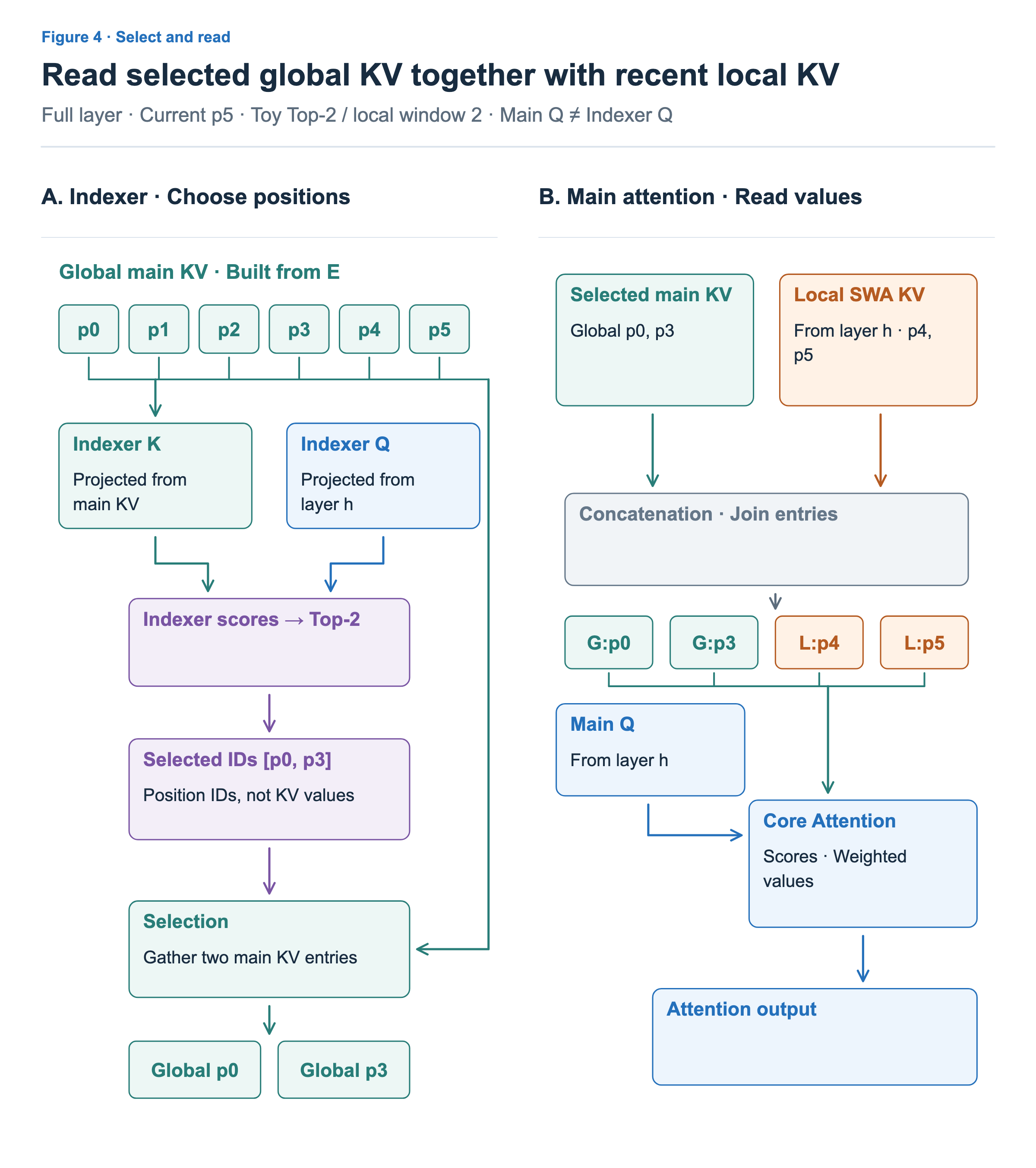
On the left, Indexer Q is produced from the current layer’s h, while Indexer K is produced from global main KV. Suppose the indexer selects [p0, p3]. This list contains the indices of positions to read. It is not yet an attention output combining the Values at those two positions.

Selection uses those indices to fetch the p0 and p3 entries from global main KV. On the right, these are concatenated with local KV for the recent positions p4 and p5. Main Q computes attention scores for these four entries and combines their Values using the resulting weights. Global KV contains values that are actually read; it is not merely information for selection. Indexer Q and Main Q have different roles and projections even though they originate from the same h.

The figure chooses non-overlapping global and local positions. This is an illustrative example, not a rule that global KV covers only older positions. Even if the same position appears in both, its KV comes from separate paths. Global KV is produced from E, while local KV is produced from h in that decoder layer.

Figure 4 in the paper likewise concatenates selected main KV with SWA KV before feeding them into Core Attention. The actual model uses Top-512 selection and an SWA window of 128. Top-2 and window 2 make the computational relationships easier to follow here.

What Full, Reindex, and Reuse Share

KV values and the list of positions to read are different objects. Layers can share the values while choosing positions again, or share both. Figure 5 compares these choices in a common layout.

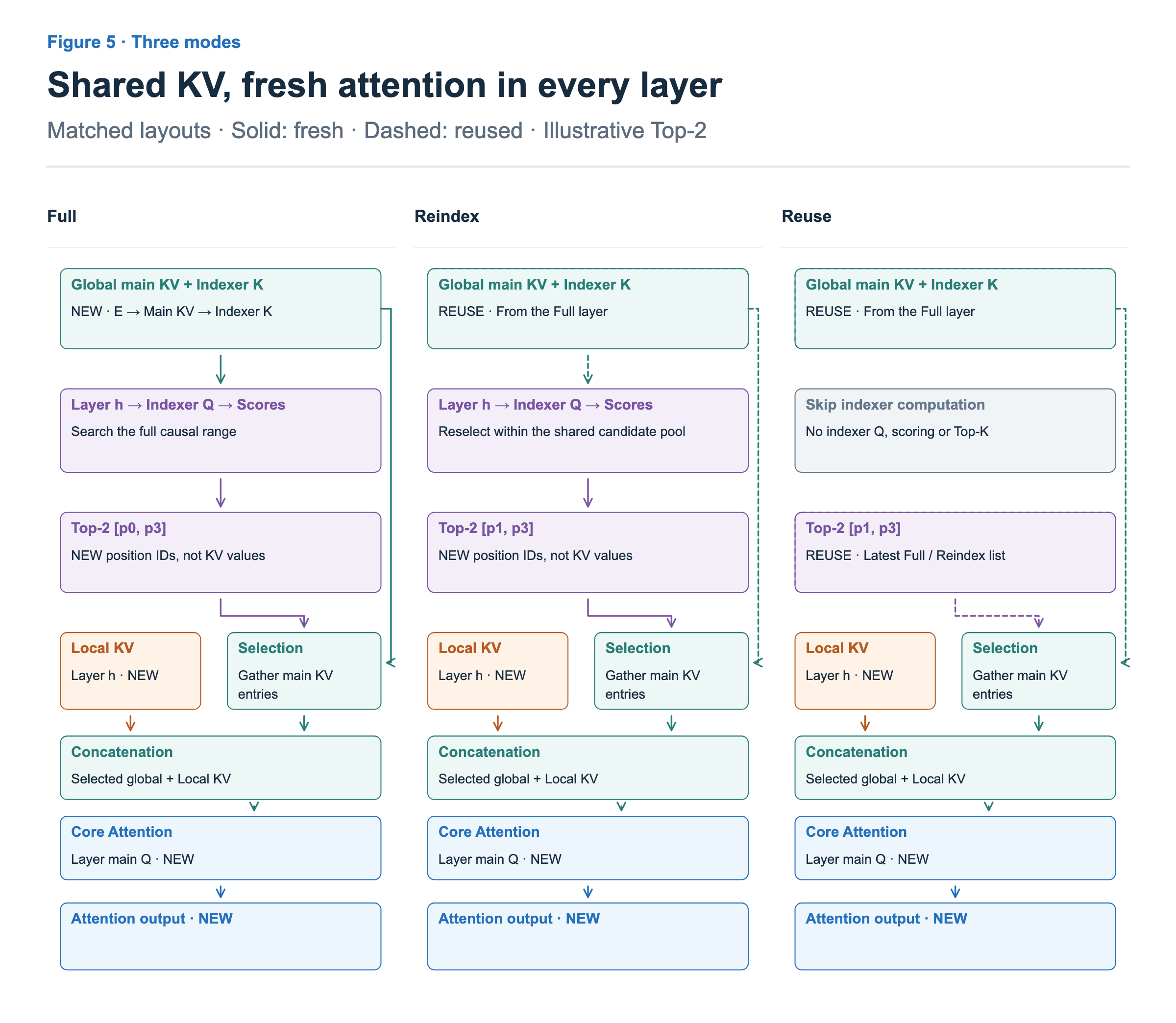
CSA2 modes are assigned to layers in advance. There is no router choosing among the three modes each time a token arrives.

• Full produces global main KV and indexer K, then computes a new selection list with its own Indexer Q.
• Reindex reads KV from the preceding Full layer but selects positions again with its own Indexer Q.
• Reuse reuses both KV and the selection list from the most recent Full or Reindex layer. It skips Indexer Q, score, and Top-K computation.

In the figure, Full selects p0 and p3, while Reindex selects p1 and p3. The subsequent Reuse layer reads p1 and p3 unchanged. However, sharing the same list does not mean copying the attention output. Every mode recomputes attention with that layer’s own Main Q and Local KV.

Reindex also has a restricted search range. The Hierarchical Sparse Indexer makes later Reindex layers choose within a shared candidate pool produced by the first Full layer. The candidate pool is a broader search set than the final Top-K list. Reindex is not simply reordering the two positions ultimately chosen by the previous layer, so it can select p1 instead of p0 as shown in the figure.

The actual 20-layer decoder begins with [Full + 3 Reuse layers], followed by four repetitions of [Reindex + 3 Reuse layers]. This totals 1 Full layer, 4 Reindex layers, and 15 Reuse layers. Figure 5 compares the three modes; it does not imply that the three modes repeatedly occur in consecutive order.

In this design, sharing KV reduces storage, while sharing selection lists reduces indexer computation. Reindex preserves the opportunity to change which positions are read without creating another KV store. Main attention and per-layer local computation continue to run.

Why Prefill Recomputes a Recent Segment

Figure 6 again uses six prompt positions, p0 through p5. The teaching example has two layers in each half and a recent replay segment W=2. Cells indicate Query positions to execute, not an attention mask.

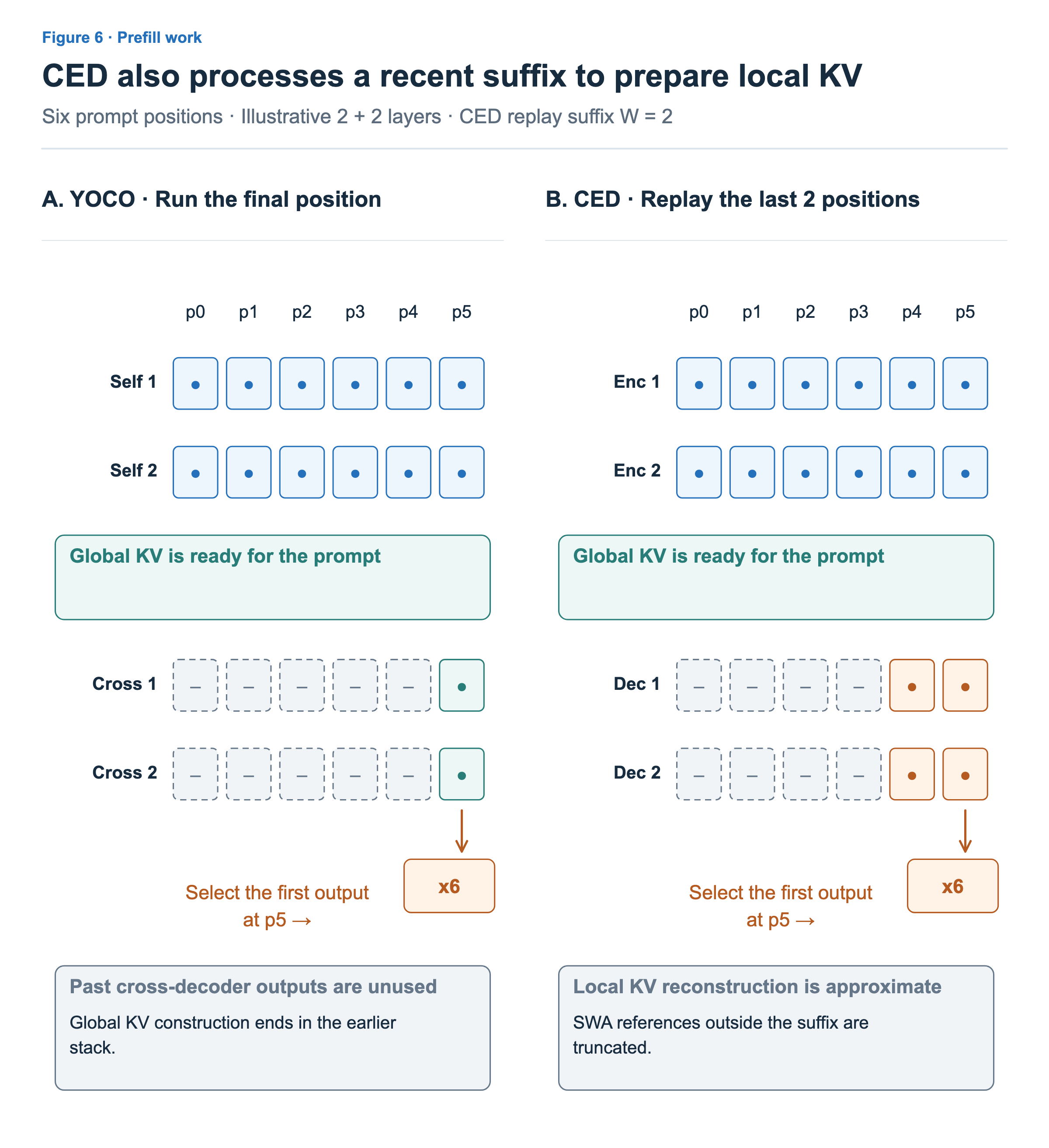
On the YOCO side, once the early layers have prepared global KV, only p5 needs to pass through the two cross-decoder layers to select the first generated token. In CED, the source of global KV is also in the early layers, but the decoder additionally needs its own local KV. The figure feeds recent positions p4 and p5 through the decoder again to prepare this state.

There is an accuracy boundary here. Bounded replay of only a recent segment does not reconstruct a state mathematically identical to a full decoder execution. Section 3.2.2 of the report constructs an approximate state by truncating SWA references outside the replay segment.

Why does computing exactly one window’s worth of positions not automatically make this exact? Consider an illustrative layer that reads the two most recent positions. The representation at p4 read by the second layer at p5 may have been influenced by p3 in the first layer. If replay starts at p4 and blocks earlier local references, the representation at p4 may already differ from a full execution. Dependencies accumulate across layers.

Bounded replay accepts this difference in exchange for reducing the remaining decoder computation over a long prompt.

After selecting the first output, the selected token becomes a new input and passes through both the encoder and decoder. Each layer updates its local state, and decoder global KV produced from E at the new position is also appended.

Together, the three articles establish clear points of comparison. CLA asks how many layers read the same KV. YOCO asks whether shared KV can be prepared without past outputs from the later layers. CED asks what state is required by its encoder-based global path and the decoder’s own local path. To decide which computation can be skipped, we must identify not only the scope of reuse but also who must produce the state needed later.