Inference Optimization for RL Rollouts

In the previous article, we saw how separating the progress of generation and training lets the learner use experience that is ready first. Now let us reduce the cost of the generator itself. RL produces multiple responses to the same question, repeatedly reads long contexts across turns, and continually updates the generation policy with trained weights. These characteristics set the conditions for inference optimization.

This article covers three directions: reducing the input that must be recomputed, advancing multiple requests together within memory, and verifying multiple candidate tokens with one policy computation. We will distinguish the costs each method reduces from the additional work it requires, then connect this to how we should think about caches and drafts in RL, where the policy keeps changing.

Reusing Computation for the Same Prefix

The phase in which the model processes the input context is called prefill, and the subsequent phase of generating tokens one at a time is called decode. The attention KV cache stores the keys and values of already processed tokens for reuse in later computation.

When generating multiple responses to one question, as in GRPO, prefixes such as the question and system instructions repeat. If the token IDs and computation conditions of this shared prefix match, sharing the KV values already computed can reduce the cost of repeatedly processing the input.

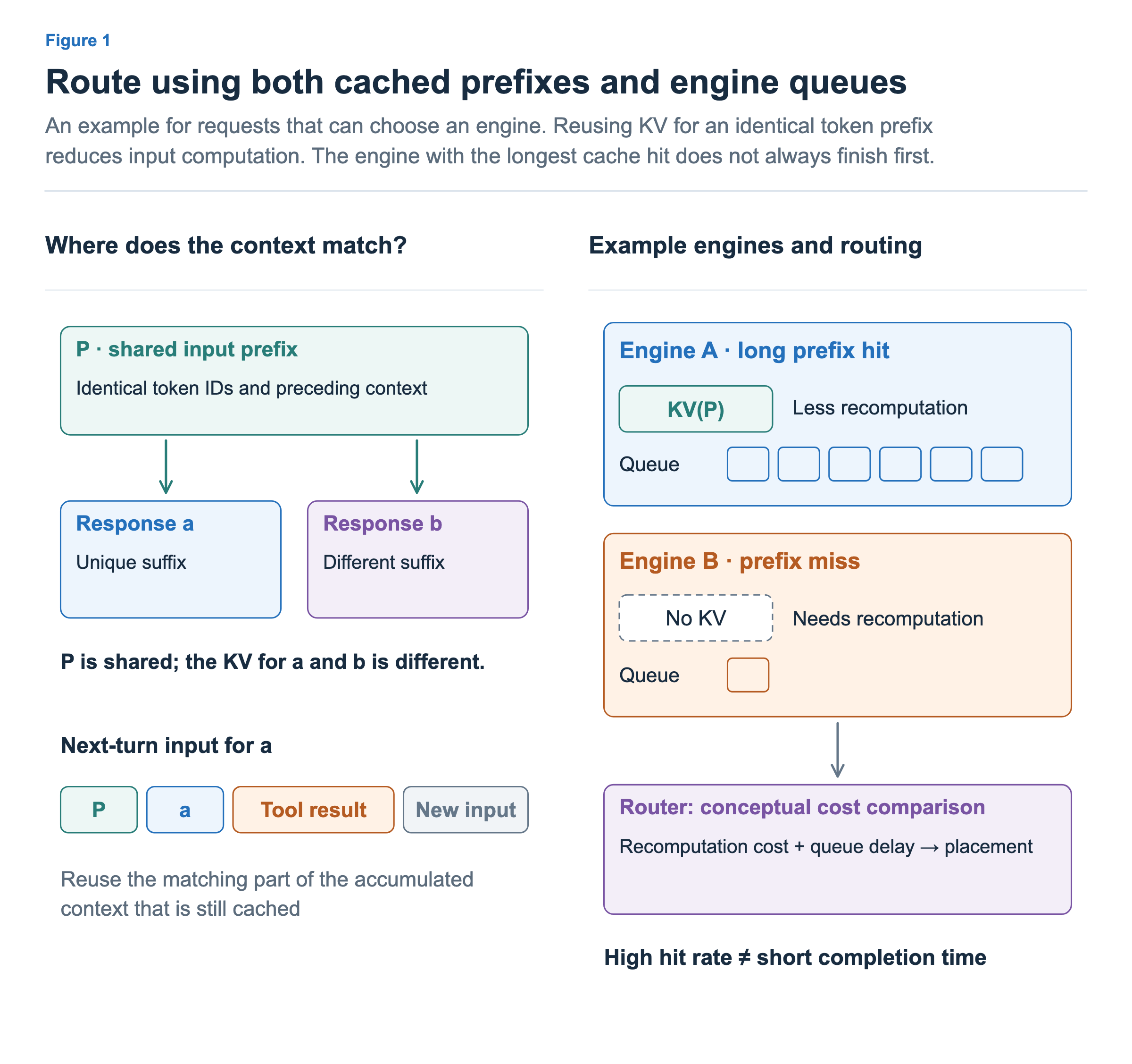
The two responses a and b in the figure share P but differ in their subsequent tokens. KV accumulated while generating a therefore cannot simply be reused for b’s different suffix. Nor does the same word appearing in the middle of a sentence imply the same KV. What preceded that token affects the computation.

In a multi-turn interaction, the context can grow into P + response a + tool observation + new input. We reuse only the beginning that is actually still cached and matches exactly. The new observation and new input still need to be processed. SGLang’s RadixAttention is a representative approach to managing this prefix KV reuse. SGLang paper

Which engine receives the request also matters. Engine A in the figure has the long prefix cached but a long queue. Engine B must recompute it because it lacks the cache, but is less busy. Continuing to send requests to A based only on the cache can reduce recomputation while increasing waiting.

Cache-aware routing decides which inference engine receives a request by considering both reusable input computation and engine load. The figure’s “recomputation cost + waiting cost” is a conceptual expression to explain the decision, not a claim that every router computes that formula literally. The router here is also the component that sends requests to inference engines. It has a different role from the MoE expert router in article 7. Miles v0.1 §2.1

Considering Free Slots and KV Capacity Together

RL responses have different lengths. When a short response finishes, a new request can join the ongoing work instead of waiting for the remaining long responses. This uses resources by continually changing the batch composition of requests being generated.

However, the number of concurrent requests alone cannot determine whether to admit new work. Long responses keep accumulating KV cache during generation, and new requests must also perform prefill to process their inputs. Freeing an execution slot and freeing KV memory are related, but they are not the same condition.

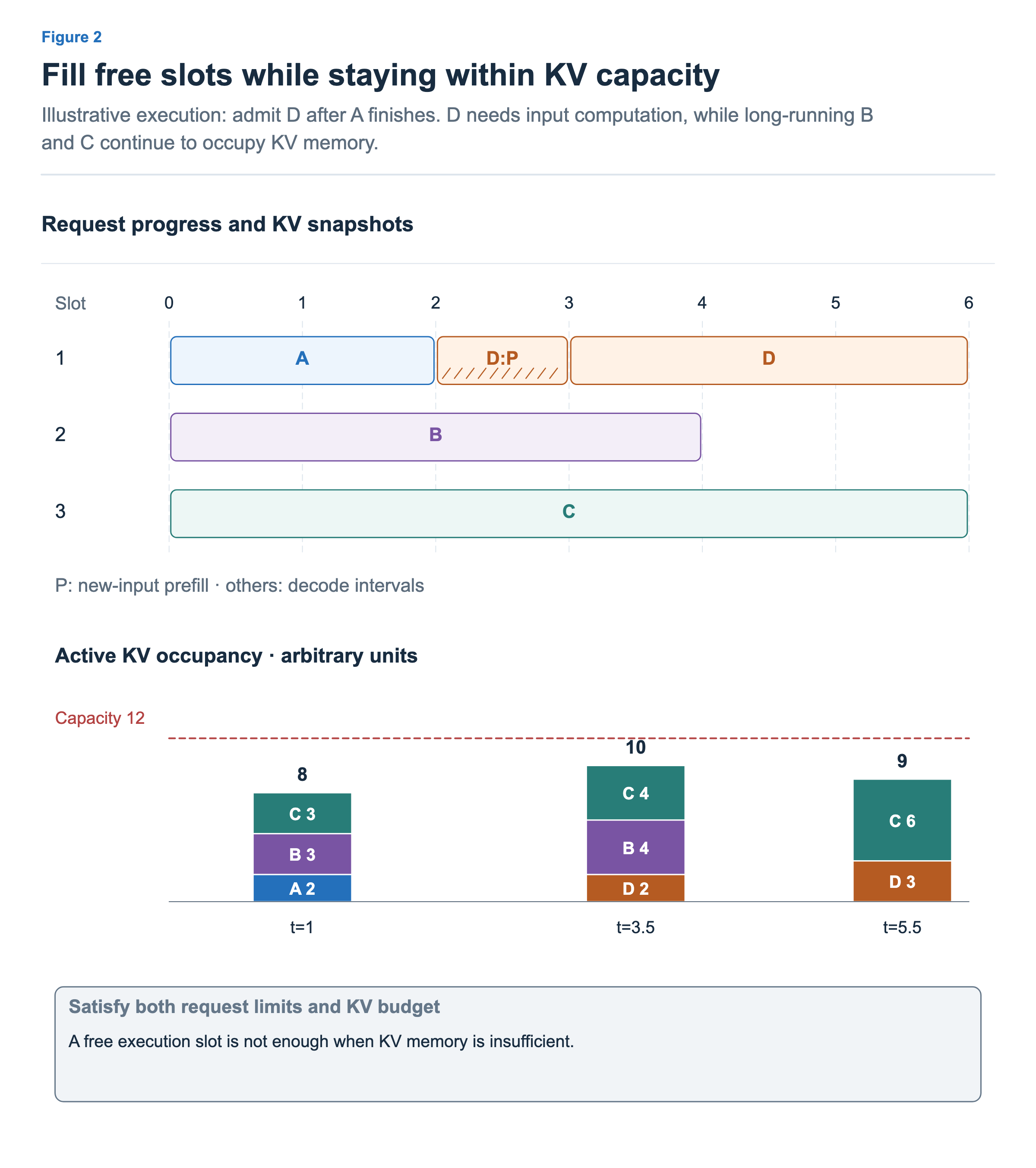
In the figure, A finishes at time 2 and D enters. D processes its input from 2–3, then generates from 3–6. B finishes at 4 and C at 6. The timeline shows intervals during which requests are in progress; it does not mean that every overlapping interval’s GPU kernels execute simultaneously.

At time 1, active KV occupancy is 8, comprising 2 for A, 3 for B, and 3 for C. At 3.5, it is 10, comprising 2 for D, 4 for B, and 4 for C. After B finishes, at 5.5 it is 9, comprising 3 for D and 6 for C. Even if the number of requests decreases, the remaining long responses’ KV grows, so total occupancy does not decrease in the same proportion.

All of these values fit within the capacity of 12 in this example. In practice, even if the maximum request-count limit is satisfied, a request must wait or another memory-management strategy must be used if the required KV memory cannot be secured. PagedAttention manages KV in blocks to reduce wasted memory. It does not eliminate the physical KV capacity limit. Actual memory management also includes retained prefix caches and other reserved space omitted from the figure. PagedAttention paper

Admitting many new requests can make their prefill compete with the decode of existing requests for the same execution resources. This is why inputs may be processed in chunks or the allocation between the two phases adjusted. Prefill and decode can also be separated onto different GPUs, but that is not a required part of this figure. In RL, we need to connect this not only to the latency of an individual output token but also to when a group becomes ready for training.

Model architecture also affects these choices. Architectures that compress KV change the storage requirement, while sparse attention can change attention computation and access patterns. However, using sparse attention does not by itself mean that all retained KV shrinks in the same proportion. Resource budgets must be based on the current model’s cache structure.

Verifying Multiple Candidates at Once

In autoregressive generation, the next token must be finalized before the token after it can be selected. Speculative decoding makes this process more efficient by combining a fast proposer with verification by the target policy.

The draft first proposes several candidate tokens. The target is the generation policy we actually want to use; it computes multiple positions along the proposed path together to verify the candidates. Verification here is not about judging correctness or assigning rewards. It determines whether a candidate can be accepted under the target’s generation procedure.

We will first follow the proposal and verification flow, then look at MTP as one way to produce candidates in the next section.

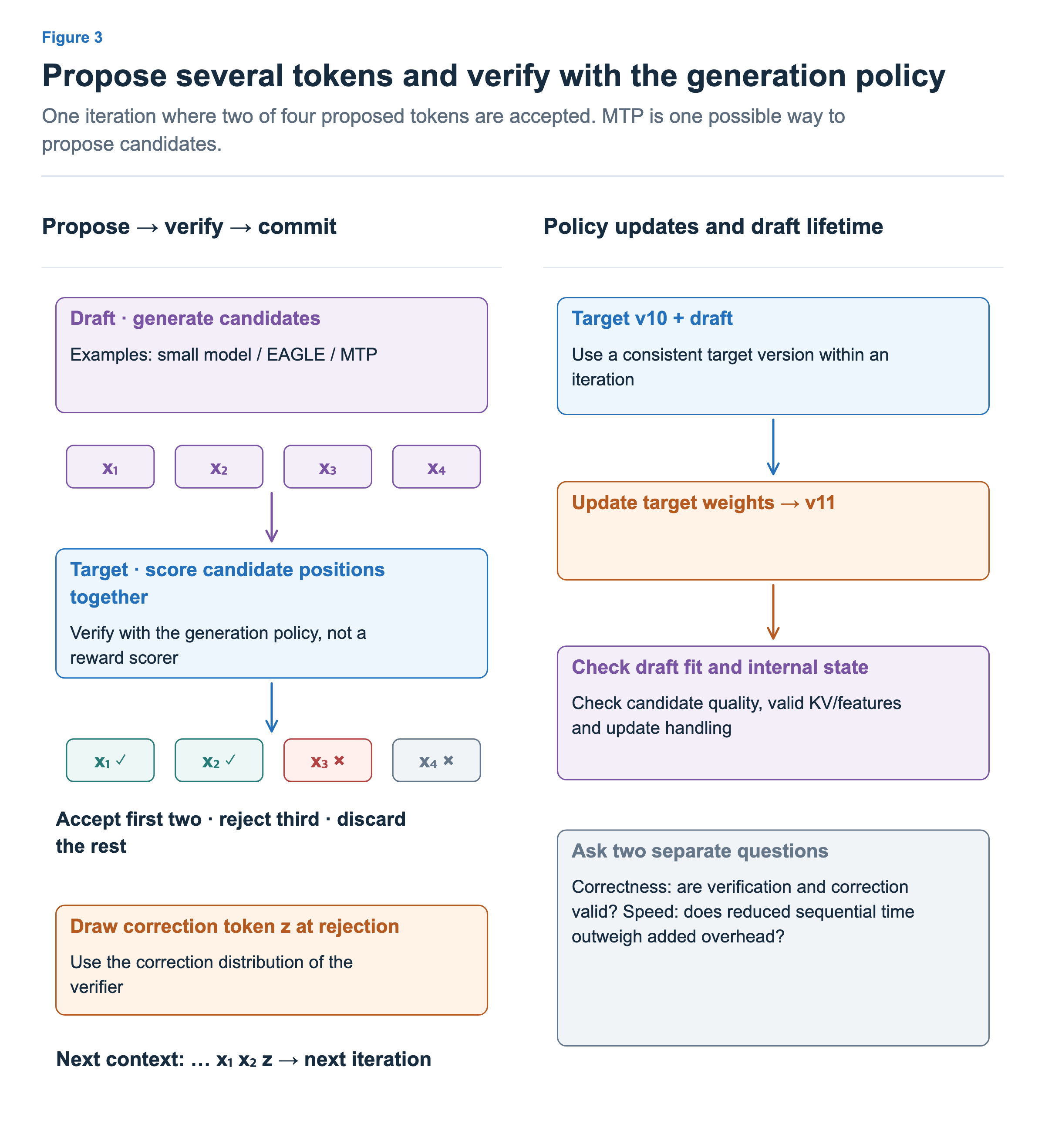
In the figure, the draft proposes x₁, x₂, x₃, x₄. Target verification accepts the first two but rejects x₃. Then x₄ cannot simply be carried forward either, because it was proposed in a context that included the rejected x₃. At the rejection point, z is sampled from the specified correction distribution, and generation starts again after the finalized x₁, x₂, z.

For stochastic sampling, this verification differs from merely checking whether both models assign the highest probability to the same token. Classical speculative sampling computes an acceptance probability using the probabilities the target and draft assign to the candidate in that context. On rejection, it samples a token from a correction distribution based on the difference between the two distributions. The probabilities here must reflect the actual sampling rules, such as temperature and top-p. When this procedure is carried out validly, multiple tokens can be advanced while preserving the target distribution. Original Speculative Decoding paper

The draft therefore does not need to imitate the target perfectly. However, poor proposals are rejected more often, reducing the work saved. Correctly preserving the distribution and actually running faster are different questions. Total computation can even increase. Acceleration comes from verifying multiple positions together while reducing sequential target calls and repeated weight and KV reads. Speed must be judged with draft generation, target verification, post-rejection handling, and additional memory costs included.

MTP Is One Way to Produce Candidates

There are several ways to build a draft. It can be a separate small model, an EAGLE-family module that uses the target’s internal features, or MTP integrated into the model.

MTP (Multi-Token Prediction) refers to architectures and training methods that predict multiple future tokens. It can be used to propose candidates during inference. Rather than counting “using speculative decoding” and “using MTP” as two completely independent acceleration techniques, it is easier to understand their relationship by asking which proposal method is used within the verification structure.

The presence of an MTP module does not mean that every inference path performs exact stochastic verification. We need to inspect the implementation’s candidate structure and verification procedure. Nor does a model providing MTP mean that the capability to train the target and draft together during RL has been publicly released.

Checking Caches and Drafts After Policy Updates

Unlike a typical service with a fixed model, RL continually updates the target policy. Cache and draft lifetimes are therefore tied to model versions as well.

First, we should not assume that KV produced with old weights can be used exactly with new weights. Even for the same tokens, changing the weights can change the keys and values. We need to check the implementation’s handling rules, such as invalidating or recomputing old caches after weight sync. Settings such as temperature, which apply only to selection after logits, should be distinguished from settings that themselves change the earlier KV computation.

There are two issues with the draft. One is how well its proposals match the tokens preferred by the new target. If the target changes from v10 to v11, an old draft’s acceptance rate can fall. The other is whether internal state that used target features or KV remains valid under the new version. Being able to retain the draft weights is different from being able to reuse its internal state unchanged.

If valid verification and correction procedures are maintained, a less well-matched draft primarily affects speed. However, if the target version changes within one verification iteration, or the probabilities and state used for verification become misaligned, the conditions for preserving the distribution can themselves be broken. Applying a new target, handling verification in progress, and clearing internal state must be coordinated consistently.

In NeMo RL research, an EAGLE-3 draft was pretrained on task rollouts and held fixed during RL in the main experiment. In measurements of Qwen3-8B-Base trained with synchronous GRPO on 32 GB200s, generation time fell from 100.0 seconds to 56.6 seconds, while the full step fell from 151.2 seconds to 107.5 seconds. This shows why a generation speedup of approximately 1.77× differs from a full-step speedup of approximately 1.41×. These are measurements for that model, task, and hardware, not expectations for every RL setup. NeMo RL research §3.1–3.2, Tables 1–2

In the same study, further training the draft during RL was a separate experiment. With a draft initialized to match the task well, the rollout speedup was nearly unchanged: 1.77× with a fixed draft and 1.78× with further training. With initialization from general conversation data, it improved from 1.51× to 1.63×. Rather than requiring the draft to be trained after every target update, the decision should depend on current acceptance efficiency and update costs. The official implementation provides a path for training EAGLE-3 by reusing features and distributions from the policy’s forward pass while detaching gradients. Study §3.3, NeMo RL EAGLE-3 guide

When examining optimization results, we can distinguish proposal length, actual accepted length, generation time, and total RL time in sequence. A longer mean accepted length may not make generation faster if draft costs also grow. Even if generation becomes faster, the overall gain is limited if training or weight transfer becomes the bottleneck.

In the next article, we will look at the lifetime of an agent program that extends beyond one model call. We will connect this to scheduling decisions about which contexts to retain in memory while tools run and which jobs to temporarily move out and restore later.