Training · 2026-10-05
One training step: from forward to a weight update
Follow next-token probabilities into loss, separate wgrad and xgrad during backward, and see an optimizer change weights through small numerical examples and a real model.
In the structure of an LLM, we followed input tokens into vectors and through layers that produce logits, the scores for the next token. Inference uses those scores to select a token. Training evaluates the probability assigned to the target and uses that evaluation to change the model’s weights.
This article follows one training step. Forward produces predictions, which are compared with targets to calculate loss. Backward computes how sensitive that loss is to each weight; the optimizer uses those results to write new weights. We will pay particular attention to how backward separates gradients for the current layer’s weights from gradients passed to the preceding layer.
The flow of one training step
Suppose the model has read I like. In inference, we select a continuation token and append it to the input. If the training sentence is I like AI, the next target AI is already known, and we can evaluate the probability the model assigned to it.
Figure 1 shows the full path from this evaluation to a weight change. Orange represents loss and gradients; purple represents the optimizer update.
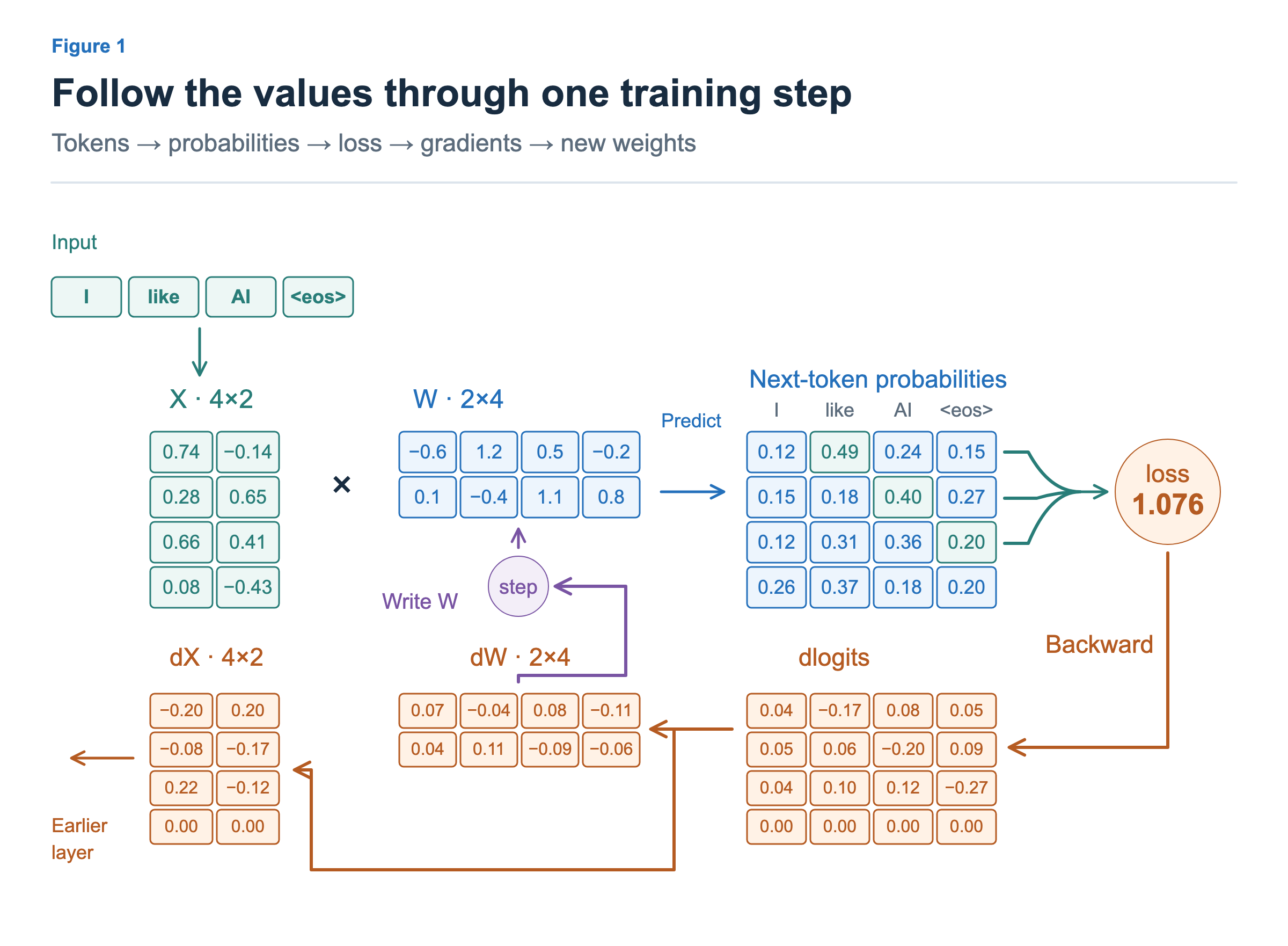
Forward predicts with the current weights; backward produces gradients for changing them. The optimizer update is what actually changes weight values. Calling loss.backward() does not finish a training step.
The figure’s numbers come from a small CPU example that makes the calculations easy to follow. Its vocabulary has only I, like, AI, and <eos>, and it omits attention that mixes context. These numbers do not measure real LLM quality or GPU performance. Later, a separate Hugging Face model confirms that the same four stages connect in a real model.
Each position predicts the next token
Forward outputs more than the last position’s prediction. Four input tokens produce vocabulary-wide logits at each position. For batch size B, input length T, and vocabulary size V, the output shape is [B, T, V].
Generation uses the last input position’s logits. Training instead connects each position’s output to the target at the very next position. Figure 2 uses input positions as columns and vocabulary entries as rows. Teal cells mark the probability of the target at each position.
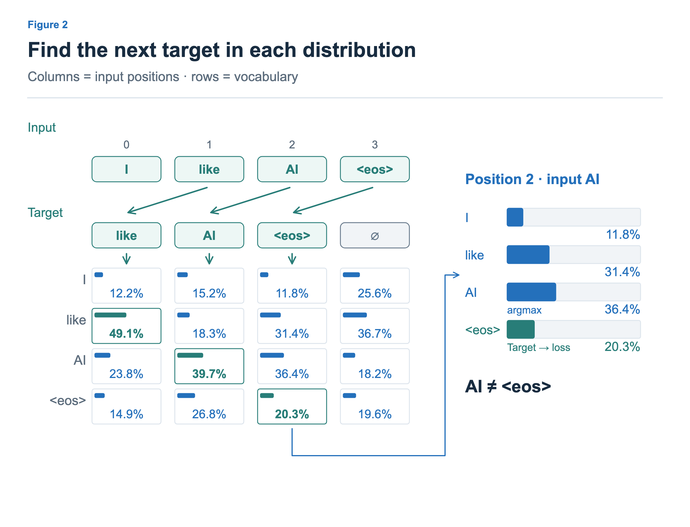
In a real causal LLM, position 0 reads I and predicts like. Position 1 reads I like and predicts AI. Position 2 reads I like AI and predicts the document-end token <eos>. The final <eos> position also has an output, but no following target exists in this example, so it does not contribute to loss.
Even when the entire target sentence is in the input, a position cannot read future tokens. Causal attention allows it to read only the current and preceding positions. Position 1, which must predict AI, cannot peek at the AI input at position 2. The small CPU model in the figures has no attention, but a real causal LLM needs this boundary.
During training, preceding inputs come from the data rather than the model’s generated tokens. Supplying the target prefix to predict the next token is called teacher forcing. One forward pass can compute predictions for many positions together. Hugging Face’s causal language modeling guide uses the same next-token prediction objective.
At position 2 in figure 2, AI has the highest probability, but <eos> is the target. Training does not merely ask whether the highest-probability token is correct. It uses the probability assigned to the target token. Even when argmax is correct, a target probability of 0.51 is evaluated differently from 0.99.
Turn target probabilities into loss
Let p be the probability assigned to the target. We need an evaluation that gets smaller as p grows and larger as p shrinks. Next-token training uses cross-entropy, or CE loss: the negative natural logarithm of the target probability.
Loss is zero when the target probability is one. At 0.5 it is about 0.693, and at 0.1 about 2.303. Assigning almost no probability to the target produces a large loss. The curve in figure 3 shows this relationship.
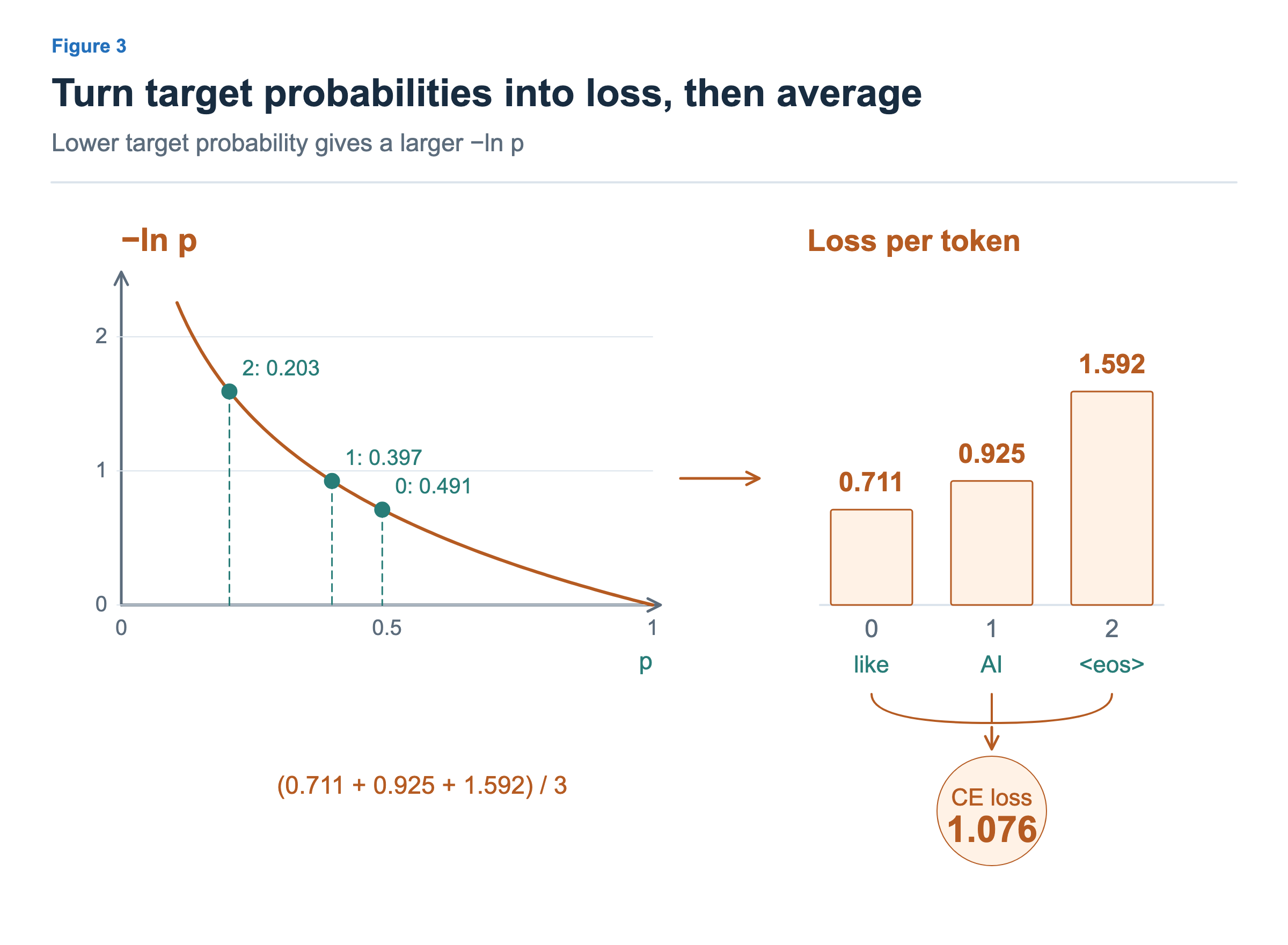
The three selected target probabilities in figure 2 are approximately 0.491201, 0.396573, and 0.203472. Their negative logarithms give token losses of about 0.710903, 0.924894, and 1.592225. Their mean is 1.076007, rounded to 1.076 in the figure.
The denominator is three valid targets, not the input length of four. Positions without targets, such as the last position, and padding positions are excluded from both the sum and denominator. The preparation articles cover document boundaries and padding; here we use one unpadded document.
For clarity, the figures convert logits into probabilities and select target cells. Actual code calculates CE stably from logits, rather than taking the logarithm of probabilities directly. Selecting a token through argmax or sampling is not part of loss calculation. PyTorch’s cross_entropy takes vocabulary logits and target IDs.
import torch.nn.functional as F

# logits: [B, T, V], input_ids: [B, T]
# One document, no padding
prediction = logits[:, :-1, :]  # No next target for the last position
answer = input_ids[:, 1:]       # The next input token is the target
loss = F.cross_entropy(
    prediction.reshape(-1, prediction.shape[-1]),
    answer.reshape(-1),
)
Aligning predictions and targets one position apart is called a shift. Passing labels=input_ids to a Hugging Face causal LM performs this alignment inside the model. Compare manually calculated CE with its internal loss, and avoid passing already-shifted labels through the internal-shift path a second time.
Backward passes gradients to earlier layers
Loss is one number evaluating a prediction. That number alone does not tell us which of the many weights to change, or by how much. We need to know how loss changes when each value changes a little. A gradient gives this sensitivity through differentiation.
A positive gradient for a weight cell means that a very small increase in that weight, with other conditions fixed, increases loss. A negative gradient means the reverse. The gradient describes this sensitivity; it is not itself a change to add directly to the weight.
Gradients first arise on the logits side. Raising the target probability lowers loss; lowering it raises loss. Differentiating softmax and mean CE together gives the following gradient for each logit at a valid position. N is the valid-target count, and the target indicator is one for the target vocabulary entry and zero otherwise.
Here, is the logit for vocabulary entry v at position t, its probability, and the target indicator described above.
For example, at position 2 in figure 2, the <eos> logit gradient is (0.203472 − 1) / 3, about −0.265509. This gradient is produced on the output side. To determine how weights inside the model contributed, we follow each operation backward.
Figure 4 uses a separate example with two linear layers to show this path. It leaves out a real Transformer’s attention, normalization, and activation functions. Its output gradient [0.1, −0.2] is a supplied value for the two-layer derivative example, not a value taken from the preceding CE calculation.
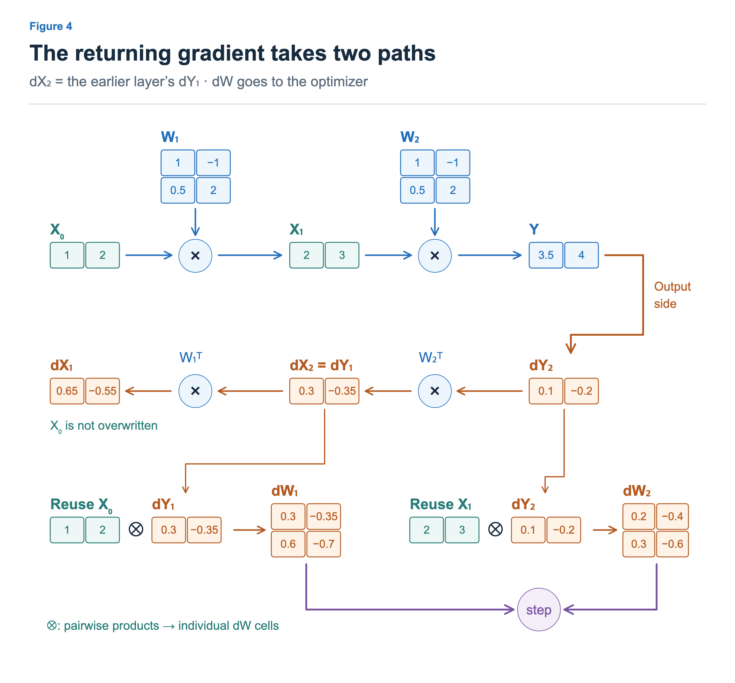
The second layer computes two things from its incoming output gradient: wgrad for its weights and xgrad for its input. That input is the first layer’s output, so the second layer’s xgrad becomes the first layer’s output gradient directly. The connection dX₂ = dY₁ in the figure expresses this relationship.
The first layer similarly computes its wgrad and xgrad. Each wgrad stays available for the optimizer; each xgrad is passed to the preceding computation. This is the chain rule, connecting the loss’s influence back to earlier weights. Layers do not pass around the loss value itself. Each receives a derivative with respect to its output and converts it into derivatives with respect to its inputs and weights.
In PyTorch, loss.backward() follows the operation relationships recorded during forward to perform these calculations. The starting derivative for a scalar loss is one. Gradients propagate through intermediate tensors and accumulate in each trainable parameter’s .grad. PyTorch’s autograd notes explain this computation graph and the intermediate values it saves.
Separate wgrad and xgrad within one layer
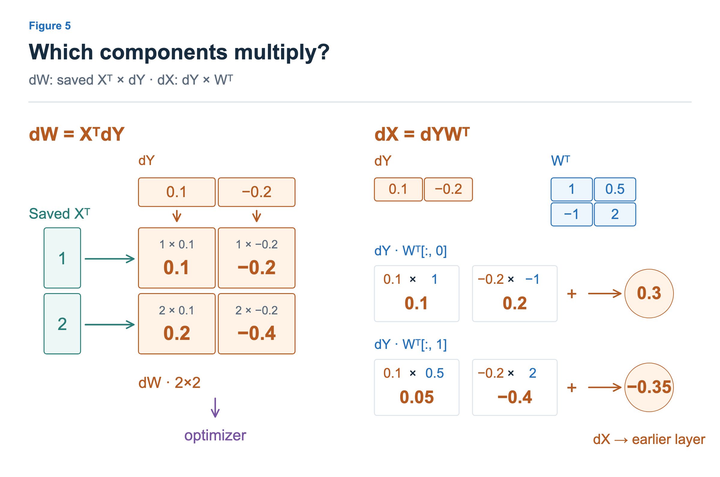
Let us expand one linear layer. We use row-vector inputs and write Y = XW. X contains input components, W weights, and Y outputs. dY is not the numeric loss; it is the loss gradient with respect to each component of output Y. Likewise, dW and dX are gradients with respect to W and X.
Figure 5 uses X = [1, 2] and W = [[1, −1], [0.5, 2]], producing Y = [2, 3]. Suppose dY = [0.1, −0.2] arrives for this output.
The gradient for W: XᵀdY
Consider the two weights connected to the first input component, 1. That input component scales each weight’s contribution to the output by one. Multiplying it by output gradients 0.1 and −0.2 gives the first row [0.1, −0.2]. The second input component is two, so its row is [0.2, −0.4].
Xᵀ is a 2×1 column vector and dY a 1×2 row vector. Multiplying every pair of components produces a 2×2 matrix: an outer product. Each result cell corresponds to the same cell in the weight matrix. With multiple input rows, their contributions are summed. In general, X of shape N×I and dY of shape N×O produce dW of shape I×O through matrix multiplication.
This calculation needs the input X from forward. dY alone does not tell us how strongly each input component scaled the weight’s influence. This is one reason an earlier activation is still needed for backward after forward ends.
The gradient for the preceding layer: dYWᵀ
Now collect the first input component’s influence on both outputs. It contributed to the first output through weight 1 and to the second through weight −1. Adding those two paths gives 0.1 × 1 + (−0.2) × (−1) = 0.3.
For the second input component, the result is 0.1 × 0.5 + (−0.2) × 2 = −0.35. Thus dX = [0.3, −0.35].
The figure’s right side places dY on the left and Wᵀ on the right, matching the formula. Wᵀ’s first column [1, −1] contains the weights connected to the first input component, and its second column [0.5, 2] those connected to the second. Multiplying each column by dY and summing produces one component of dX. This calculation needs the current layer’s weights W.
Computing dX does not overwrite X with a new value. If X is an activation from the preceding layer, dX becomes that layer’s output gradient so backward can continue. The trainable objects are the parameters reached along that path. Input token IDs are not changed by gradients either. Gradients accumulate in trainable parameters such as embedding tables as the necessary paths toward the input are followed.
You can compare these calculations in code. Instead of starting from loss, this example passes an already-arrived dY to y.backward(dy).
import torch

x = torch.tensor([[1., 2.]], dtype=torch.float64, requires_grad=True)
w = torch.tensor([[1., -1.], [.5, 2.]],
                 dtype=torch.float64, requires_grad=True)
dy = torch.tensor([[.1, -.2]], dtype=torch.float64)
y = x @ w

y.backward(dy)

dw = x.detach().T @ dy
dx = dy @ w.detach().T
torch.testing.assert_close(w.grad, dw)
torch.testing.assert_close(x.grad, dx)
print(w.grad)  # [[0.1, -0.2], [0.2, -0.4]]
print(x.grad)  # [[0.3, -0.35]]
Both explicit formulas had zero maximum absolute error against autograd in this example. A displayed floating-point value of 0.3 may internally be stored as approximately 0.30000000000000004, so comparisons use torch.testing.assert_close.
Actual torch.nn.Linear stores weights in [output component, input component] order, transposed relative to this article’s W in [input component, output component] order. Calling the stored weight A, forward is X @ A.T, stored-weight wgrad is dY.T @ X, and xgrad is dY @ A. Match these orientations when comparing the figures’ formulas with .weight in real code.
So far we have expanded a linear layer. Other operations, such as activation functions and attention, can require different saved values for backward. This does not mean every operation only needs to save its input X. The next article observes when these values appear and when they are no longer needed in memory.
The optimizer writes new weights
After backward, gradients have the same shapes as the parameters. Every parameter value has a corresponding gradient value. But a gradient is different from the actual weight change. The optimizer applies a learning rate and its algorithm’s rules to determine the update.
Figure 6 returns to the initial CPU example and follows one cell, W[0,1]. Before forward its value is 1.2. After backward it is still 1.2, now with gradient −0.0384565.
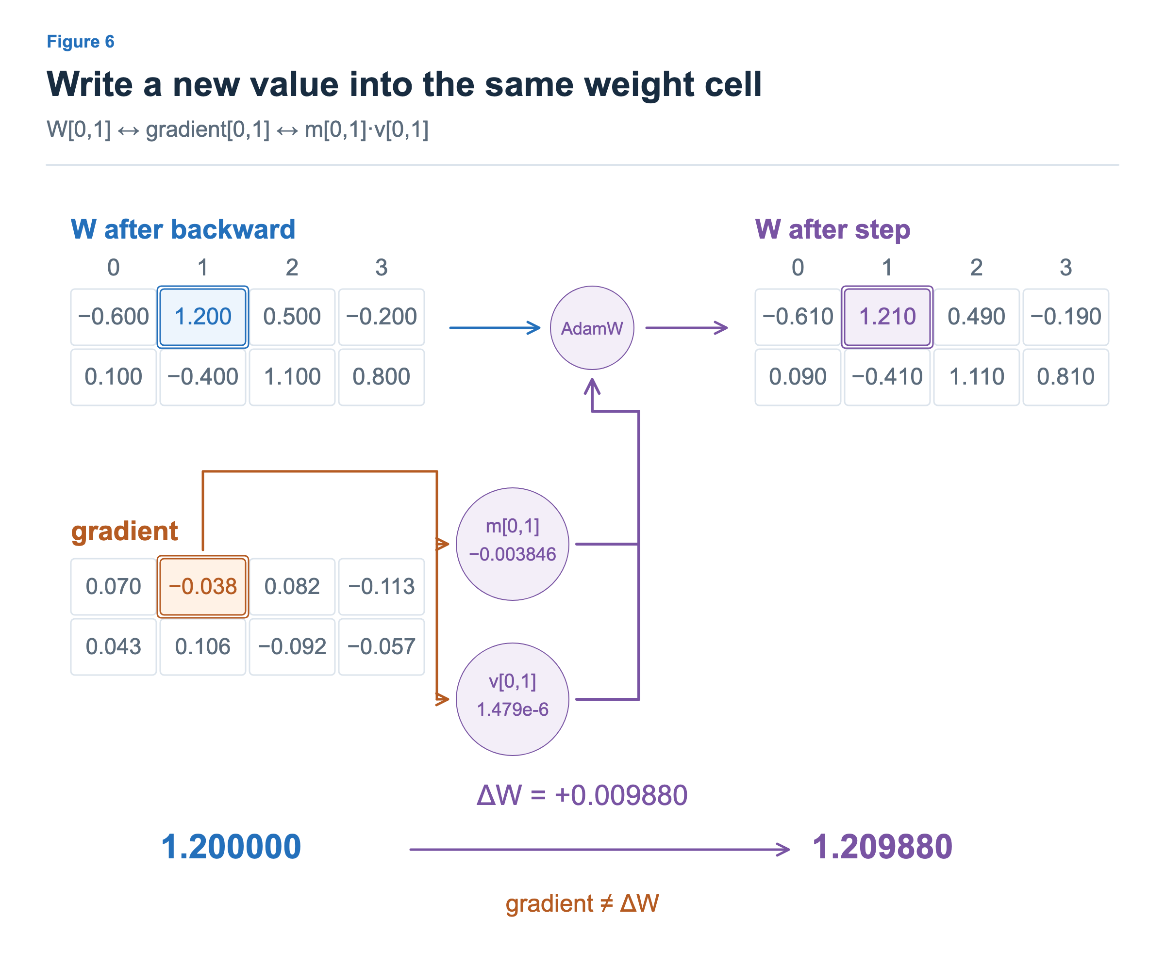
After AdamW’s step(), the same cell is approximately 1.209880: an actual change of about +0.009880. This is not the result of adding gradient −0.0384565 directly to the weight. The figure uses a learning rate of 0.01 and weight decay of 0.01.
AdamW uses not only the current gradient but also state maintained for each parameter. m is an average that accumulates gradient direction; v is an average that accumulates squared gradients. Both begin at zero, then incorporate each new gradient into the preceding step’s state. The figure’s m/v values are the states updated for this step and used in its weight update. These states help explain why a current gradient and the actual update are not identical. Chapter 4 expands the m/v and weight-decay calculations in AdamW’s official definition.
The training code should show this order:
optimizer.zero_grad(set_to_none=True)
outputs = model(input_ids=input_ids, labels=input_ids, use_cache=False)
loss = outputs.loss
loss.backward()
optimizer.step()
zero_grad() clears the preceding step’s parameter gradients. PyTorch accumulates backward results into existing .grad values, so a step that needs fresh gradients requires this boundary. Here, one backward is followed by one update. Chapter 3 covers gradient accumulation across several backward passes.
Check one step in a real model
Now check that the same path connects in a real model. The lab uses pretrained HuggingFaceTB/SmolLM2-135M, chosen so a short CPU input can expose all parameter gradients and an AdamW update. The preparation articles’ baseline uses a GPT-2 tokenizer, but does not load GPT-2 weights. It pretrains our GPT-style decoder from random initialization on FineWeb. This chapter instead uses SmolLM2 to observe pretrained next-token predictions immediately.
Model and tokenizer are pinned to revision 93efa2f097d58c2a74874c7e644dbc9b0cee75a2. The run used Python 3.12.8, PyTorch 2.8.0, and Transformers 4.57.1, with CPU FP32 computation. This chapter does not introduce mixed precision or execution optimization.
Generate the next token from the last position
First, input I like and select one token with the highest probability at the last position. We use argmax to keep the generation rule simple.
import torch
from transformers import AutoTokenizer, AutoModelForCausalLM

model_id = "HuggingFaceTB/SmolLM2-135M"
revision = "93efa2f097d58c2a74874c7e644dbc9b0cee75a2"
tokenizer = AutoTokenizer.from_pretrained(model_id, revision=revision)
model = AutoModelForCausalLM.from_pretrained(
    model_id, revision=revision, dtype=torch.float32,
    attn_implementation="eager",
)
model.eval()
inputs = tokenizer("I like", return_tensors="pt", add_special_tokens=False)
with torch.no_grad():
    logits = model(**inputs, use_cache=False).logits
    next_id = logits[:, -1, :].argmax(-1, keepdim=True)
    generated = torch.cat([inputs.input_ids, next_id], dim=1)
print(tokenizer.decode(generated[0]))  # I like to
The selected token in this run was ID 288, to, producing I like to. We could append the generated to to continue generation, but the training example below uses the data’s target AI instead of that generated result.
model.eval() changes layer behavior such as dropout, while torch.no_grad() disables gradient recording. These are separate roles. Training forward does not use no_grad(), and the model is switched to train() mode.
Compare per-position CE with the model’s loss
The training input is I like AI followed by EOS, with IDs [57, 702, 5646, 0]. The tokenizer represents them as I, Ġlike, ĠAI, <|endoftext|>; Ġ marks a preceding space. The figures use <eos> as a simplified name for this document-end token. The actual vocabulary size is 49,152, giving logits of shape [1, 4, 49152].
| Input position | Input token | Next target | Target probability | Token CE |
|---|---|---|---|---|
| 0 | I |
Ġlike |
0.00126005 | 6.676604 |
| 1 | Ġlike |
ĠAI |
0.00002470 | 10.608803 |
| 2 | ĠAI |
<|endoftext|> |
0.00084043 | 7.081603 |
| 3 | <|endoftext|> |
None | Excluded | Excluded |
Mean CE over the three valid targets is 8.122337. The difference between manually shifted CE and the model’s internal loss from labels=input_ids was zero in this run. The figures’ 1.076007 comes from a different model; these loss magnitudes are not a model-quality comparison.
The complete lab also records each position’s top five probabilities and the remaining probability mass. At position 1, for example, Ġto was most probable at approximately 0.274680, but loss used the target ĠAI’s probability. These actual outputs connect the displayed distribution to the training objective.
Check a representative linear layer’s gradient and update
We observed down_proj in the first decoder block’s MLP. Its input X has shape [1,4,1536], its output gradient dY [1,4,576], and its stored weight A [576,1536]. Combining batch and position into four input rows lets us compare dA = dY.T @ X and dX = dY @ A.
The lab’s hook observes this layer’s forward input and output, and retain_grad() exposes intermediate gradients. This is instrumentation; ordinary training does not require separately retaining every activation’s .grad. Both matrix formulas had zero maximum absolute error against the observed gradients in this run.
After backward, we selected a weight cell with a nonzero gradient and recorded its update. The following values describe this model’s actual stored weight A[507,1365]. This is a different cell from W[0,1] in figure 6, and its learning rate is also different, at 0.0001.
| Observation point | Weight value | Gradient |
|---|---|---|
| Before forward | 0.484375000 | None |
| After backward | 0.484375000 | +0.311700791 |
| After AdamW step | 0.484274536 | +0.311700791 |
The entire observed weight matrix was exactly unchanged before and after backward. After the step, the selected cell changed by about −0.000100464. Optimizer steps do not automatically clear .grad, so the same gradient remains in the final row. The next step’s zero_grad() clears it.
This run verifies the connection between predictions, loss, gradients, and weight changes. One update on one sentence does not demonstrate improved validation performance or language ability. Later technique comparisons will evaluate learning with shared training data and separate validation data.
The independent code is labs/training/chapters/01-forward-backward/train.py. Install its dependencies and run from the repository root. The first run downloads the public model.
python -m pip install -r labs/training/chapters/01-forward-backward/requirements.txt
python labs/training/chapters/01-forward-backward/train.py --device cpu
The default output, results/chapter-01.json, records per-position probabilities, token losses, gradient comparisons, and parameter changes. --device cuda runs on a GPU, but the values above are CPU results, not measurements of GPU throughput or memory.
Next: lifetimes of values needed for computation
Forward made predictions with the current weights. After target probabilities became loss, backward computed wgrad and xgrad in each layer. xgrad went to preceding layers, while the optimizer used parameter gradients to write new weights.
Computing wgrad required the activation from forward again. Where did that value live between forward and backward, and when was it no longer needed? The next article uses memory snapshots and timelines of the same training path to observe activations accumulating, being used, and being released.