MQA and GQA: Sharing KV Across Queries

In Q·K·V projections and Core Attention, we followed how each head gathers information using its own query, key, and value. In that arrangement, increasing the number of query heads also increases the number of corresponding key and value heads.

When generating tokens one at a time, we can store keys and values from earlier positions for reuse. As the context grows, however, there are more values to store. Could multiple queries use the same keys and values to reduce storage while preserving the computation that gathers information for each query?

This article first compares the sharing patterns of three structures. We then trace how one token leads to computation across multiple heads in MHA, before extending the example to MQA, where all query heads share KV, and GQA, where sharing occurs within groups. Finally, we examine exactly what becomes smaller, by how much, and the resulting trade-offs.

Connecting queries to KV

MHA (Multi-Head Attention) uses a separate key head and value head for each query head. MQA (Multi-Query Attention) shares one key head and one value head across multiple query heads. GQA (Grouped-Query Attention) divides query heads into groups and shares keys and values within each group.

We will use KV to refer to keys and values together, and one KV head to mean a corresponding pair of one key head and one value head. The following figure compares four, two, and one KV heads while keeping four query heads.

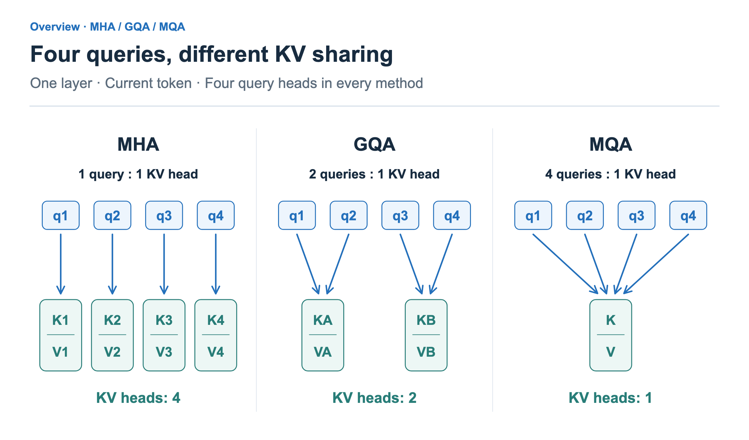
The vectors $q_1$ through $q_4$ are the query vectors computed by the current token’s four query heads. They are not queries from four different tokens. Each KV set below them represents the keys and values those queries will access. The arrows show which KV set each query uses.

In MHA, the mapping is one-to-one: $q_1$ uses $K_1/V_1$, $q_2$ uses $K_2/V_2$, and so on. In GQA, shown in the middle, $q_1$ and $q_2$ share $K_{\mathrm{A}}/V_{\mathrm{A}}$, while $q_3$ and $q_4$ share $K_{\mathrm{B}}/V_{\mathrm{B}}$. In MQA, all four queries use the same $K/V$. All three structures have four query heads; what changes is the number of KV heads and the scope of sharing. This comparison redraws the GQA paper’s architecture diagram with four query heads.

MHA: separate KV for each head

Consider processing the current position $p_3$ in one layer. Positions $p_0$, $p_1$, and $p_2$ precede it, so there are four token positions to attend to, including the current position. The number after $p$ denotes a position in the context, rather than a token type or a head number.

For a small example, let the model dimension be 8, the number of query heads be 4, and the dimension of each head be 2. Keys and values also have two components per head. We will keep these conditions throughout the figures. These are illustrative dimensions, not measurements from an actual model.

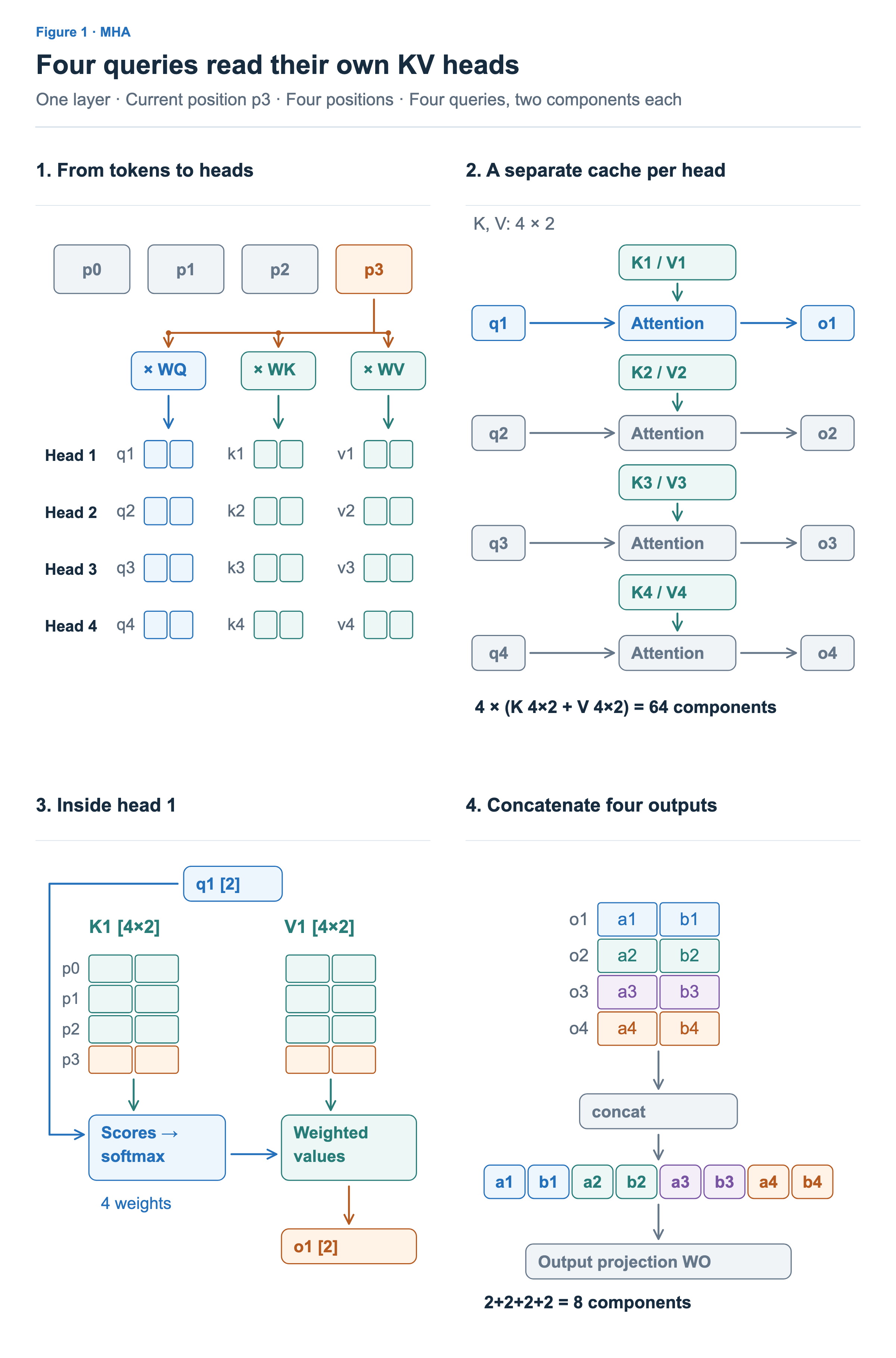
In the first panel of Figure 1, each block from $p_0$ to $p_3$ represents one input vector at that position. It is the vector entering this layer, not a single vector component. We multiply the entire eight-component vector at the current position $p_3$ by three different weight matrices, $W_{\mathrm{Q}}$, $W_{\mathrm{K}}$, and $W_{\mathrm{V}}$, to produce Q, K, and V.

In this MHA example, each projection produces eight components. Grouping them into four heads with two components each gives $q_1\dots q_4$, $k_1\dots k_4$, and $v_1\dots v_4$. Each small cell below represents one vector component, and each row represents one head. For example, $q_1$, $k_1$, and $v_1$ are all vectors for Head 1 at the current position. We do not first split the input vector into four pieces and send one piece to each head. Each head projects the entire input using different weights.

Suppose we have kept the keys and values for $p_0$ through $p_2$ before computing the current position. This storage of keys and values from processed positions is the KV cache. Adding the newly computed $k_1$ and $v_1$ to Head 1’s cache leaves $K_1$ and $V_1$ containing four positions, from $p_0$ through $p_3$. The other heads add their current-position values in the same way.

Here, lowercase $k_1$ and $v_1$ denote vectors at the current position, while uppercase $K_1$ and $V_1$ denote matrices collecting multiple positions. Each matrix is four positions × two components per head, or $4\times 2$. Moving down one row means moving to the next token position; switching from $K_1$ to $K_2$ means using another head’s representation.

The third panel expands Head 1’s computation. Taking the dot product of the two-component $q_1$ with each of the four rows of $K_1$ produces four position scores. Applying the scaling and softmax described in Core Attention produces four weights that sum to 1. The current position $p_3$ can attend to every position from $p_0$ through itself.

Using those weights to take a weighted sum of the four rows of $V_1$ gives the two-component output $o_1$. Here, the weights are the proportions determined by this query for incorporating the value at each position. They are distinct from the learned parameters $W_{\mathrm{Q}}$, $W_{\mathrm{K}}$, and $W_{\mathrm{V}}$ used to produce Q, K, and V.

The other three heads similarly compute $o_2$, $o_3$, and $o_4$ using their own queries and KV. Concatenating the four outputs gives $2+2+2+2=8$ components, which the output projection $W_{\mathrm{O}}$ combines. Labels such as $a_1$ and $b_1$ in the figure represent the two components of each output vector.

Keys and values from past positions are reused when computing the next position, but past queries do not need to be stored in this KV cache. The new position’s query reads the stored keys and values. We can now consider reducing the number of KV sets stored in this computation.

MQA: sharing KV across all queries

In MHA, each head produced its own keys and values at every position. MQA produces one key vector and one value vector per position and shares them across all query heads. Queries are still produced separately for each head.

At the current position $p_3$, the Q projection still produces four queries with two components each. The K and V projections, however, each produce only two components. With a model dimension of 8, this configuration has an $8\times 8$ matrix $W_{\mathrm{Q}}$ and $8\times 2$ matrices $W_{\mathrm{K}}$ and $W_{\mathrm{V}}$.

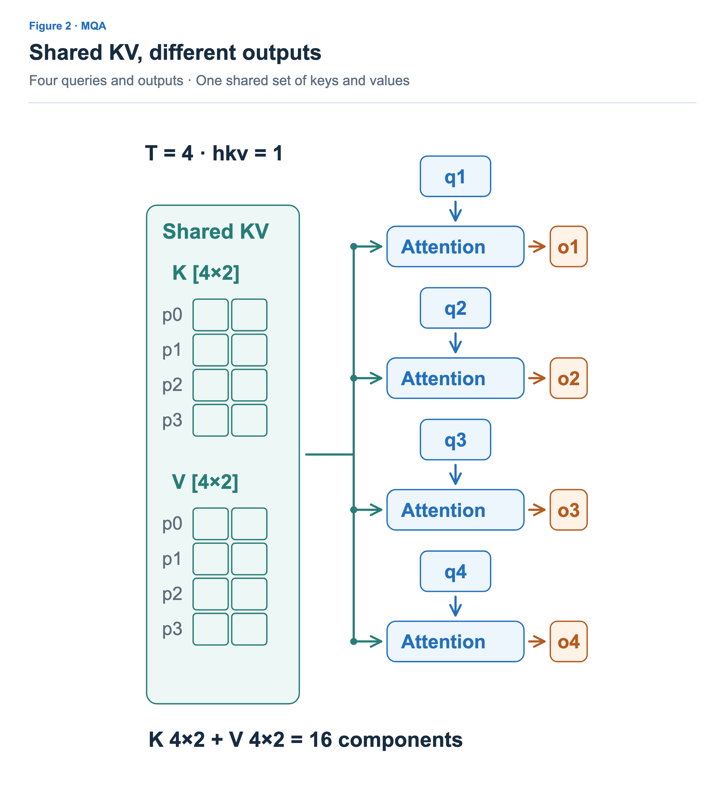
The left side of Figure 2 contains one K matrix and one V matrix, each of size $4\times 2$. Having one KV head does not mean storing only one token position. The shared K and V still contain values for all four positions, from $p_0$ through $p_3$.

On the right, $q_1$ computes scores using the four rows of K, applies softmax, and takes a weighted sum of V to produce $o_1$. The query $q_2$ uses the same K and V, but its different query vector can produce different position scores and weighting proportions. For example, one query may give more weight to the value at $p_0$, while another gives more weight to the value at $p_2$.

Thus, sharing the same KV does not force the outputs to be identical. Each of the four queries performs its own attention computation and produces its own output. The four Attention boxes distinguish these computation relationships; they do not require four separate kernel launches. As in MHA, the outputs are concatenated and passed to the output projection.

Storage changes substantially. MHA stores four sets of K and V, while MQA stores just one. In this example, that is $K4\times 2+V4\times 2=16$ components. By sharing KV across heads, MQA reduces the amount of KV to store and read during token-by-token generation. MQA paper

GQA: sharing KV within groups

GQA defines the scope of KV sharing by group. If we divide four queries into two groups, the first contains $q_1$ and $q_2$, and the second contains $q_3$ and $q_4$. Each group uses a separate K and V.

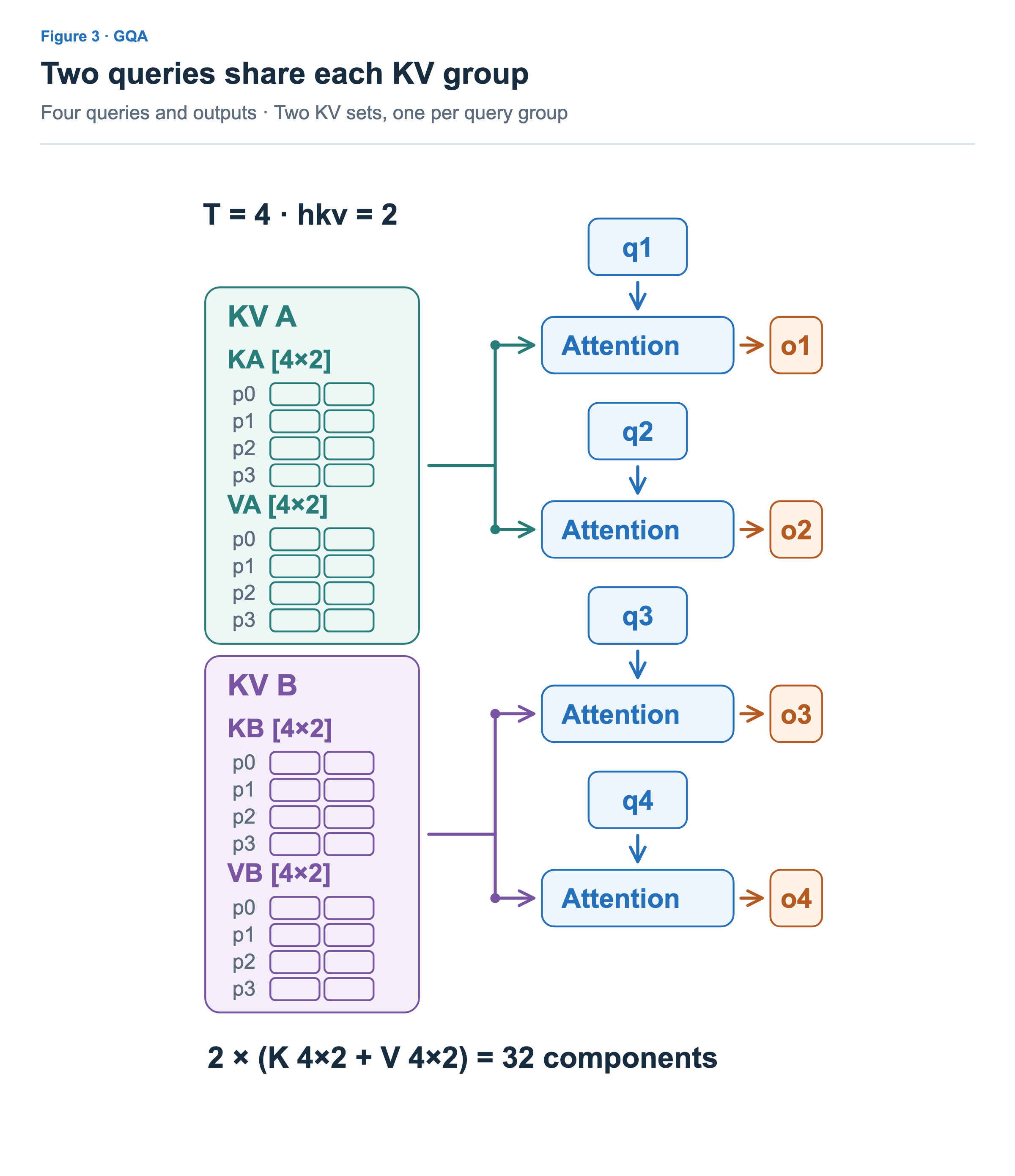
In Figure 3, $q_1$ and $q_2$ both read $K_{\mathrm{A}}/V_{\mathrm{A}}$, while $q_3$ and $q_4$ both read $K_{\mathrm{B}}/V_{\mathrm{B}}$. Each group’s KV contains all four positions. The groups divide query heads, not the token positions stored in the cache.

At the current position, the Q projection still produces four queries with two components each. The K and V projections each produce two heads with two components each. In this example, $W_{\mathrm{K}}$ and $W_{\mathrm{V}}$ are each $8\times 4$, and each KV head adds its newly computed values to its corresponding cache.

Within a group, sharing works as in MQA. The queries $q_1$ and $q_2$ read the same KV but gather values using their own computed proportions. The second group follows the same process. There are still four outputs, $o_1$ through $o_4$, but only two KV sets to store. Total storage is $2\times 16=32$ components.

Let $h_q$ denote the number of query heads and $h_{\mathrm{kv}}$ the number of KV heads. In the usual configuration with equally sized groups, $h_q/h_{\mathrm{kv}}$ query heads share each KV head. In this example, that is $4/2=2$. Setting $h_{\mathrm{kv}}=1$ gives MQA’s sharing pattern; setting $h_{\mathrm{kv}}=h_q$ gives MHA’s. GQA adjusts the degree of sharing between these two endpoints. GQA paper, Section 2.2

KV head count and storage

We can now compare the three KV caches using equally sized cells. Each cell represents one stored component. All three configurations have four token positions and two components per head for both K and V.

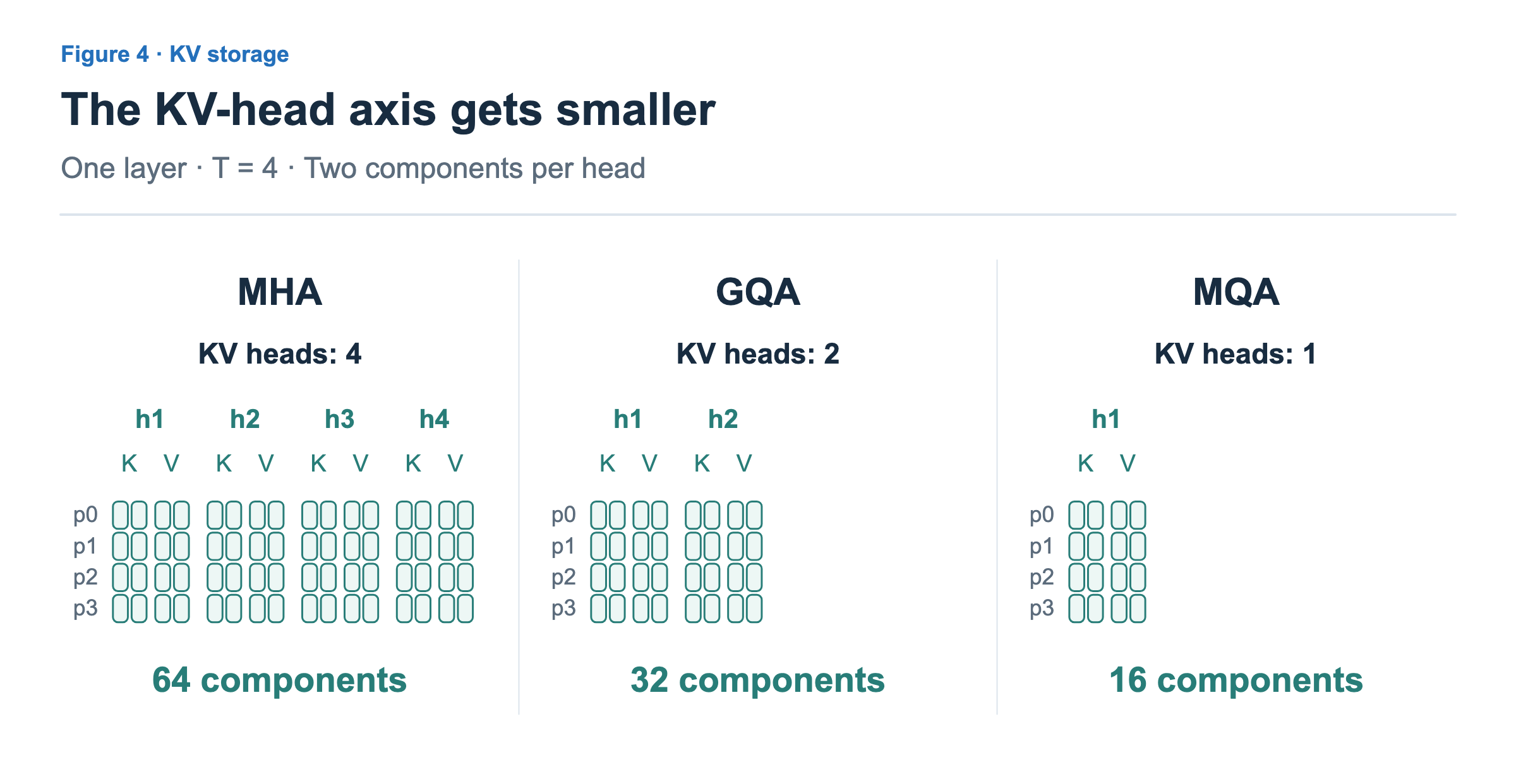
In MHA, each of the four KV heads has eight key components and eight value components, giving 64 components in total. GQA has two KV heads and 32 components; MQA has one KV head and 16. This reduction comes from storing fewer separate KV heads, while preserving the number of token positions and components per head.

For one request in one layer, we can generalize this as follows. Here, $T$ is the number of token positions in the cache, $h_{\mathrm{kv}}$ is the number of KV heads, and $d_h$ is the dimension per head. We assume equal head dimensions for K and V.

$$\text{Stored KV components}=2\times T\times h_{\mathrm{kv}}\times d_h$$

The leading 2 accounts for storing both K and V. Substituting the MHA example gives $2\times 4\times 4\times 2=64$. For GQA and MQA, only $h_{\mathrm{kv}}$ changes, to 2 and 1 respectively. With the other conditions and storage size per component held equal, GQA’s KV storage relative to MHA is $h_{\mathrm{kv}}/h_q$. In this example, GQA uses half as much storage and MQA uses one quarter.

This expression counts the KV values themselves. For an entire model, storage must be summed across layers; for multiple requests, it must also be summed across requests. Actual memory allocation may include additional space depending on the implementation.

Even with sharing, each query computes scores against the keys at the positions it attends to and takes a weighted sum of their values. Keeping the number of query heads and the context length unchanged leaves this core attention arithmetic at the same scale. Meanwhile, the output size of KV projections and the amount of KV to store decrease. An implementation that reuses shared KV effectively can also reduce the amount of data fetched from memory.

Consequently, reducing the cache to one quarter of its size does not necessarily reduce total execution time to one quarter. Other operations, model-weight reads, and how the kernel reuses KV also affect runtime. The figures 64, 32, and 16 in this article compare stored component counts.

Choosing a sharing scope

MHA can learn separate key and value representations for each query head. MQA requires all queries to use the same key and value representations; GQA applies that constraint within each group. Broader KV sharing reduces storage, but also reduces the freedom to produce different keys and values for different heads.

For this reason, arbitrarily combining KV at runtime in a model trained with MHA does not preserve its outputs. MQA and GQA are model structures with different KV projections and head connections. The GQA paper presents a method that converts the KV projections of an existing MHA checkpoint and then performs additional training. In its experiments, it reports GQA quality close to MHA and speed close to MQA. Those results apply to the paper’s models and training and execution conditions. GQA paper, Sections 2–3

When reading an actual model configuration, therefore, check both the query-head count and the KV-head count. Their ratio helps explain the sharing scope and KV storage, while quality and speed must be evaluated with the model trained for that structure and its execution environment.

We have examined how to change KV sharing while preserving per-query computation and outputs. The next article moves beyond the scope of sharing to consider making the stored KV representation itself smaller.