MLA storage: Representing KV with a small latent vector

The previous article examined MQA and GQA, which reduce cache storage by sharing KV across query heads. Now we will change the representation being stored. Instead of keeping every head’s keys and values, could we store a small vector from which they can be formed?

MLA (Multi-head Latent Attention) is a structure trained to form the keys and values of multiple heads from one small latent vector. A latent vector is an intermediate representation of the input with fewer components. This compact representation is stored, and each head uses different projections to obtain the representations it needs.

We will first see how one latent vector produces head-specific K and V. Next, we will explain why a positional key for RoPE is formed and stored through a separate path. Combining the two paths will show what differs between heads and what is shared, before we calculate cache storage as the token count grows. This article focuses on key/value representations and storage. Forming queries and computing attention scores are covered in the next article.

Forming head-specific K and V from a small vector

Suppose one layer is processing the input at the current position $p_{\mathrm{3}}$. Each block from $p_{\mathrm{0}}$ through $p_{\mathrm{3}}$ represents the entire input vector at that position. We will use an input dimension of 8, a latent dimension of 3, and two heads. Each head’s content key and value have two components. Unlike the four-head example in the previous article, we use two heads here to examine the relationship between the latent vector and its projections. All dimensions and values are illustrative.

Let $x_{\mathrm{3}}$ be the input vector at the current position, with shape 1×8. Multiplying it by the 8×3 weight matrix $W^{\mathrm{D}}$ produces a 1×3 latent vector $c_{\mathrm{3}}$. The figure assumes the result is [1, 2, 3]. The weights are learned, and D identifies the down-projection that reduces the dimension.

$$c_{\mathrm{3}}=x_{\mathrm{3}}{W}^{\mathrm{D}}$$

The subscript 3 in $c_{\mathrm{3}}$ denotes the token position, not the latent vector’s third component or Head 3. By contrast, the subscript 1 in $U_{\mathrm{1}}^{\mathrm{K}}$ and $U_{\mathrm{1}}^{\mathrm{V}}$ below denotes the head number, while the superscripts K and V distinguish the representations each projection produces. Since the current position is fixed in the figure, its subscript is omitted from the head-specific outputs.

Both heads use the same $c_{\mathrm{3}}$ but project it with different weights. For example, Head 1’s key projection $U_{\mathrm{1}}^{\mathrm{K}}$ is the 3×2 matrix shown in the figure. Multiplying [1, 2, 3] by this matrix gives 1×1 + 2×0 + 3×0 = 1 for the first output and 1×0 + 2×1 + 3×0 = 2 for the second, yielding [1, 2].

Head 1’s value projection $U_{\mathrm{1}}^{\mathrm{V}}$ combines the first and third latent components in its first output. The result is therefore [1 + 3, 2] = [4, 2]. Head 2 uses different projections to obtain the key [2, 3] and value [1, 5]. Sharing a latent vector does not make the heads’ K and V identical.

In the figure, $U_{\mathrm{1}}^{\mathrm{K}}$ and $U_{\mathrm{2}}^{\mathrm{K}}$ are the output slices for each head within the full key up-projection. The value projection can be divided in the same way. U denotes the up-projection from the latent representation to the representations of multiple heads. Separating the heads in the diagram does not require separate matrix multiplications in an implementation. This is a small row-vector example of joint KV compression in the DeepSeek-V2 paper. The weight matrices are oriented in the opposite direction from the paper’s column-vector notation.

The key point is that the model is trained to pass through a small joint representation. This does not mean that any existing model’s K and V can later be converted into three numbers and always recovered exactly. The weights that map inputs to latent vectors and those that map latent vectors to K and V are learned together. A small latent dimension reduces storage while constraining the K and V that multiple heads can represent.

Storing a positional key separately

The keys in the previous section carry a superscript C. This denotes the content part, distinguishing it from the separate RoPE path. Attention using RoPE applies position-dependent rotations to queries and keys so that their positional relationship affects the score. MLA needs this capability too.

MLA forms a positional key through a path separate from the content-key path. Figure 2 sends the input at the same $p_{\mathrm{3}}$ position through both paths and stores their outputs in a new cache row.

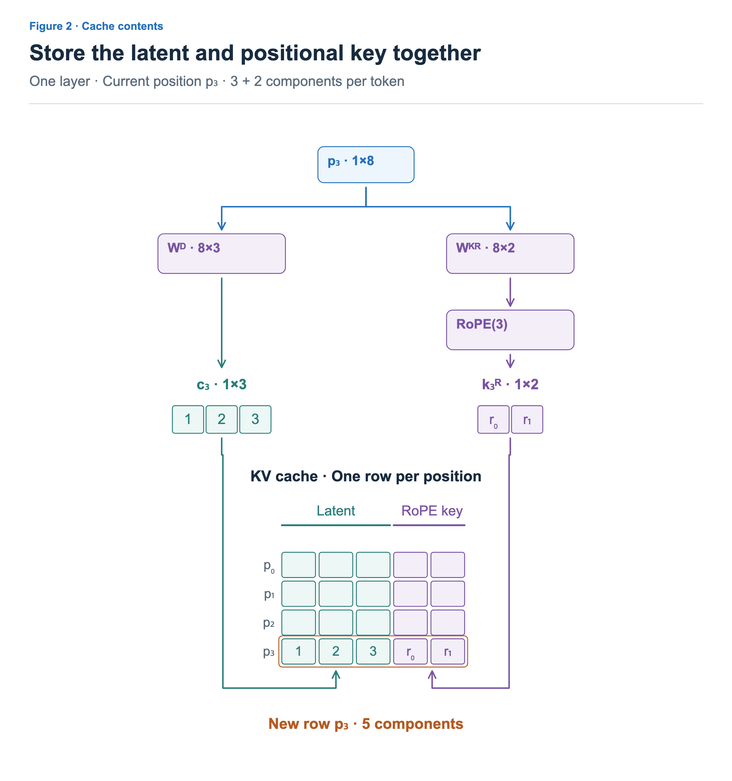
The left path uses the $W^{\mathrm{D}}$ projection introduced earlier to produce $c_{\mathrm{3}}$ = [1, 2, 3]. The right path applies a separate 8×2 projection $W^{\mathrm{KR}}$ to the input, followed by RoPE for the current position, 3. This produces the two-component positional key $k_{\mathrm{3}}^{\mathrm{R}}$. The superscript R identifies the RoPE path. The symbols $r_{\mathrm{0}}$ and $r_{\mathrm{1}}$ in the figure denote the two components of this vector, not two token positions.

One positional key is formed per token position and shared by all heads in the same layer. We do not store two separate copies of $k_{\mathrm{3}}^{\mathrm{R}}$ for Heads 1 and 2. A different position, such as $p_{\mathrm{2}}$, needs its own positional key formed from its input and rotation. Sharing is across heads; it does not merge different token positions. DeepSeek-V2 paper, Section 2.1.3

At the current position, we therefore store three latent components and two positional-key components, for a total of five. The existing rows from $p_{\mathrm{0}}$ through $p_{\mathrm{2}}$ remain, and [1, 2, 3, $r_{\mathrm{0}}$, $r_{\mathrm{1}}$] is appended as a new row for $p_{\mathrm{3}}$. The five cells group the two stored representations into one illustrated row; they do not require a single contiguous array in actual memory.

The positional path is separated to enable efficient computation with the compact stored representation. Inserting position-dependent RoPE rotations directly into content keys makes it difficult to combine the key projection with query-side operations in advance. The rotation, which varies by position, intervenes between fixed, position-independent projections. A separate positional path preserves the rearrangement of content-path computation while retaining positional relationships. The equations and order of computation are covered in the next article.

This does not mean that a latent vector cannot contain any position-related information. A layer’s input may carry contextual information from earlier computations. What is separated here is the path that explicitly applies RoPE rotations. The positional key is also formed by projecting the input and then rotating it, so it is not a fixed vector determined only by the position index.

Two paths for forming keys and values

Let us combine the head-specific projections in Figure 1 with the positional path in Figure 2. Figure 3 shows how keys and values are composed. It does not show queries or the full attention computation.

Head 1’s content key is [1, 2], and Head 2’s is [2, 3]. Concatenating the same positional key [$r_{\mathrm{0}}$, $r_{\mathrm{1}}$] to each produces the following four-component keys.

Head	Full key	Value
Head 1	[1, 2, $r_{\mathrm{0}}$, $r_{\mathrm{1}}$]	[4, 2]
Head 2	[2, 3, $r_{\mathrm{0}}$, $r_{\mathrm{1}}$]	[1, 5]

The two parts are concatenated, not added component by component. The key dimension is therefore 4: two content components plus two positional components. The value keeps its two components projected from the latent vector. The positional key is not appended to the value.

Even with the same positional part, the full keys can differ between heads because different projections form their content parts. Also, sharing a positional key does not make the positional attention scores identical across all heads. Queries also contribute to the scores, and MLA forms positional queries separately for each head. The next article will connect the content and positional query parts to the corresponding key parts.

We must also distinguish what is cached from the expanded representations in the diagram. The cache stores $c_{\mathrm{3}}$ and $k_{\mathrm{3}}^{\mathrm{R}}$ at the top. The head-specific K and V below are expanded to illustrate the keys and values that this compact representation can express. This does not prescribe an execution procedure that reconstructs and stores all past K and V in this form for every subsequent token.

The distinction becomes clear when compared with MQA. In MQA, multiple queries share the completed K and V. MLA forms head-specific content K and V from a joint latent representation and separately shares the key part used for RoPE. What is shared determines the relationship between the heads’ representations.

Cache growth with token count

A smaller per-token representation still needs to be retained for each past token position. In this MLA example, each position stores three latent components and two positional-key components. Four stored tokens require 4×5 = 20 components. Processing the fifth token adds one row, bringing the total to 25.

Let $d_{\mathrm{c}}$ be the latent dimension, $d^{\mathrm{R}}$ the positional-key dimension, and $T$ the number of stored token positions. In this configuration, which stores two small vectors instead of expanded per-head K and V, the number of values needed for one request in one layer is:

$$\text{Stored components}=T\times (d_{\mathrm{c}}+d^{\mathrm{R}})$$

Substituting our dimensions gives $T$×(3+2) = 5$T$. The positional key is shared across heads, so its dimension is not multiplied by the head count again. There is also one joint latent vector per position. The absence of an explicit head-count factor does not mean that a real model’s latent dimension can be reduced arbitrarily without regard to its heads. The latent dimension is tied to the capacity of the learned representation.

MHA and GQA from the previous article also append a new cache row for each additional token. Figure 4 reuses the MHA and GQA settings from Article 1 alongside this MLA example. In all three configurations, the upper snapshot stores four tokens and the lower snapshot stores five.

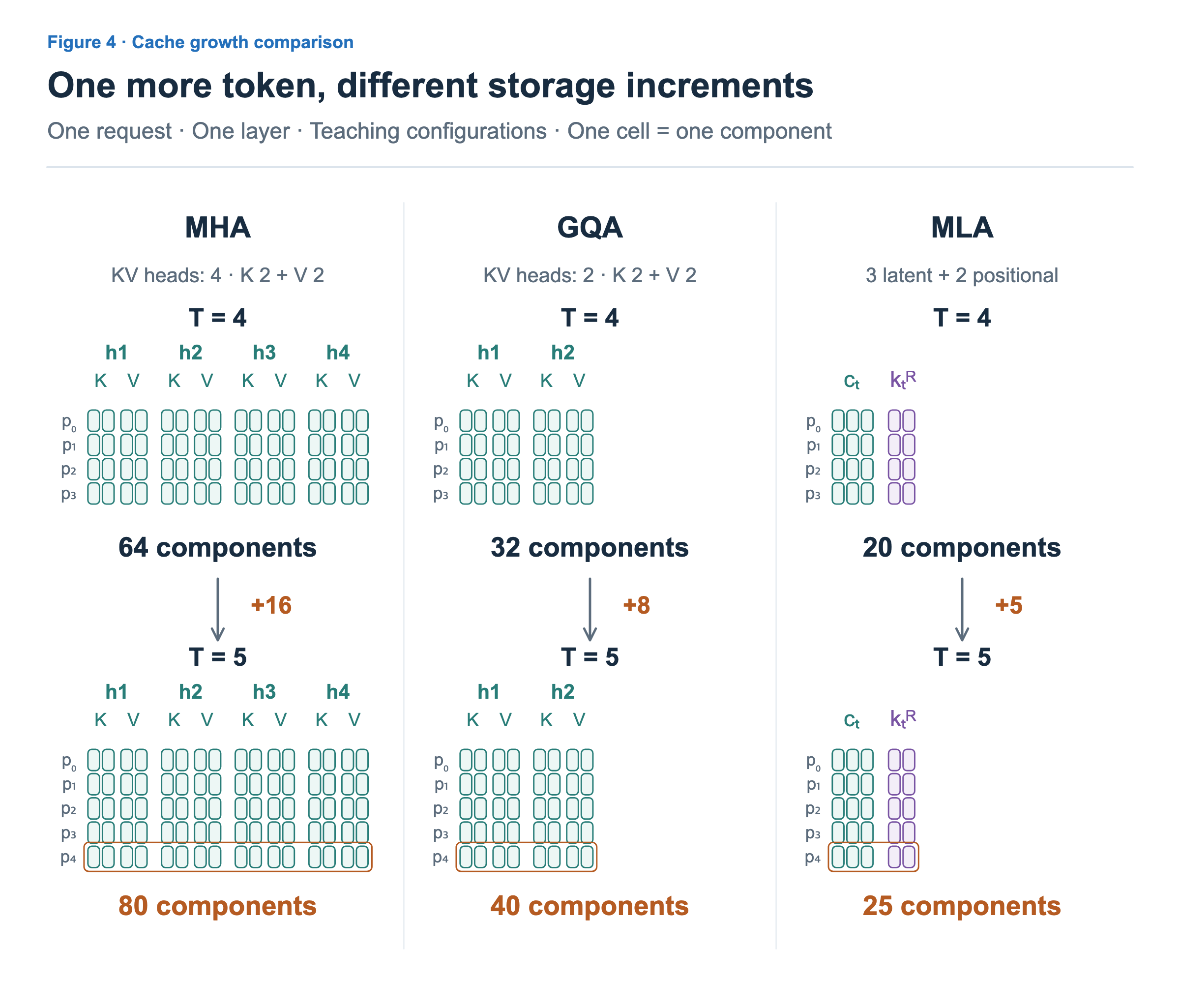
Every cell has the same size and represents one stored component. The orange outline marks the newly appended $p_{\mathrm{4}}$ row. The head labels in MHA and GQA denote KV heads.

• MHA stores two K and two V components for each of four KV heads. Each token adds 4×(2+2) = 16 components, increasing total storage from 64 to 80 components.
• GQA uses two shared KV heads. Each token adds 2×(2+2) = 8 components, increasing storage from 32 to 40 components.
• MLA stores a joint latent vector and a shared positional key. Each token adds 3+2 = 5 components, increasing storage from 20 to 25 components.

With these settings, both total storage and the per-token increment decrease from MHA to GQA to MLA. GQA reduces the number of KV heads stored; MLA stores a joint representation from which head-specific K and V are formed. The figure compares the stored representations and their sizes in the two articles’ teaching configurations. Actual savings depend on head counts and dimensions; this is not a performance comparison between models of equal quality.

The expression and figure count values stored in the cache. To obtain memory size, account for the bytes stored per component and sum across layers and requests. Weights, temporary computation space, and memory-alignment overhead are not included.

Compact storage and the remaining computation

MLA stores a compact joint representation for the K and V of multiple heads. This requires projections connecting the latent and head-specific representations, as well as a separate key for RoPE. The amount of storage saved depends on the chosen latent and positional dimensions.

The cache reduction ratio is also not the reduction ratio for total execution time. Runtime depends on how attention is computed from the compact representation, the kernels, context length, and execution environment. The remaining question is how the current query reads the stored latent vectors and positional keys. The next article will first connect the two parts of Q, then examine how rearranging the computation avoids fully expanding head-specific KV each time.