Shared Concepts · Models · 2026-09-27
MLA Computation: Attention Without Expanding KV
Follow how the current query reads a latent KV cache, and see why moving the key projection to the query and the value projection after the weighted sum preserves the result.
The previous article explained how MLA caches a shared latent vector and a positional key instead of storing every head’s keys and values. But if every new token required expanding all past K and V vectors again, reconstructing them would still take computation.
MLA can move the computation that expands K and V while preserving the result. It moves the key projection to the current query and applies the value projection after combining information across positions. This reduces repeated projections at cached positions and lets attention read the compact latent representation directly.
We will first see how the current token produces its query and how content and positional information contribute to attention scores. Then we will reorder the key and value computations to see which operations disappear and which remain. We will follow the processing of the current token in one layer during token-by-token generation.
Building queries for the current token
As before, let the current position be and the input dimension be 8. The cache contains latent vectors and positional keys for four positions, through the current . The KV latent dimension is 3, each head’s content key and value dimensions are 2, and the positional dimension is also 2. These small dimensions are illustrative.
We now build the query that will read the cache. Each block at the top of Figure 1 represents an entire input vector at one position. The lower part shows two query heads produced from .
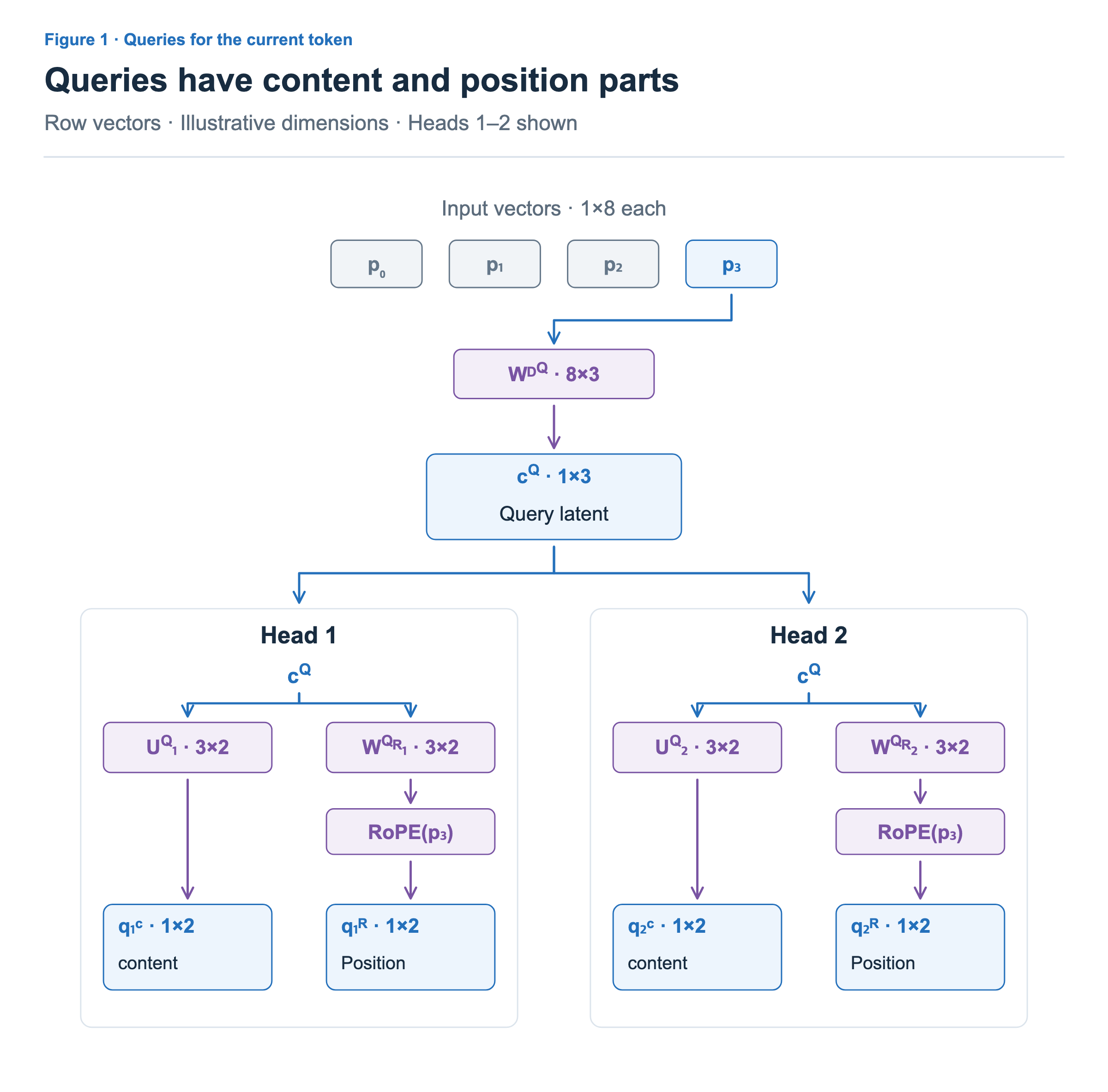
Applying the 8×3 projection to the current input produces the query latent vector . This and the cached KV latent vector from the previous article are representations produced by different weights. Both have three components in this example, but their dimensions do not have to match in an actual model.
Each head produces two kinds of query from . For head 1, the 3×2 projection produces a two-component content query. is also a 3×2 projection, but its output undergoes the RoPE rotation for the current position to produce a positional query. Head 2 uses its own weights, so both query parts differ by head. This follows DeepSeek-V2’s low-rank query projection and decoupled RoPE construction.
From here on, we will show both position and head indices. is the content query for position 3, head 1, and is the positional query for the same position and head. Superscripts C and R distinguish the content and RoPE paths. Figure 1 omits the position subscript because the current position is fixed; Figure 2 onward includes both indices.
Positional queries are per-head, whereas all heads share the positional key at a given cached position. Thus, different queries can produce different positional scores even when they read the same positional key. Queries are used to compute scores now; past queries do not need to accumulate in the KV cache.
The figure focuses on projections and positional rotation. It omits steps such as normalization of latent vectors. DeepSeek-V2’s model configuration also includes RMSNorm after latent vectors. When we combine operations below, we mean consecutive linear projections after normalization.
Adding content and positional scores
Let denote the position being read from the cache. With current position 3, can be 0, 1, 2, or 3. To read position , head 1 needs its content key, positional key, and value.
The left side of Figure 2 shows the K and V construction from the previous article; the right side shows how the current query produces a score. We will start by expanding K and V before computing attention.
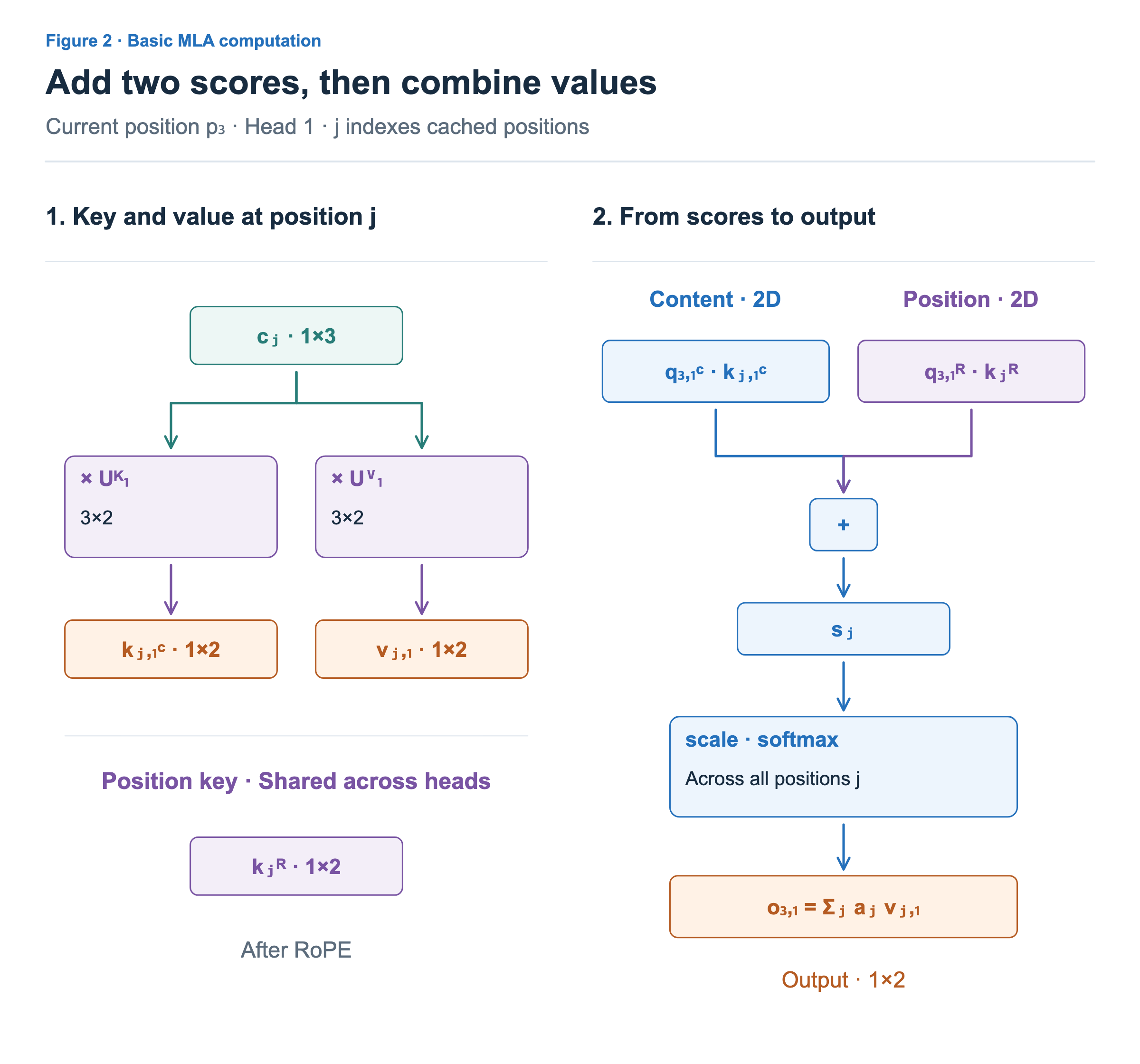
The latent vector at position has shape 1×3. Multiplying it by head 1’s produces content key ; multiplying it by produces value . Both projections have shape 3×2, and each result has shape 1×2. The separately cached positional key is also 1×2, but has no head index because it is shared across heads.
The current query and cached key take dot products between matching parts: content query with content key, positional query with positional key. Each dot product gives one number. Adding them produces score for position .
The dot symbol denotes a vector dot product. Concatenating the content and positional parts, as in the previous article, and taking one dot product gives the same result. For example, content query [2, 1] and content key [1, 2] give 4, while already-rotated positional query [1, 0] and positional key [0.6, 0.8] give 0.6. The total is 4.6. Content and positional parts are not cross-multiplied.
After computing scores for all four positions, we apply scaling and softmax. The original query/key dimension here is content 2 plus positional 2, or 4, so the basic scaling divisor is √(2+2) = 2. Dividing each score by 2 and applying softmax across all four positions yields attention weights . We do not apply softmax independently to a single score at each position.
Combining with these weights produces head 1’s output . Positional information influences how much weight each position receives, but the positional key is not appended to the value for the weighted sum. The current token can attend through its own position; when computing multiple tokens together, a causal mask must prevent them from reading future positions.
This is the basic attention computation represented by MLA. The next two sections preserve its result while eliminating the step that expands all per-head K and V vectors.
Moving the key projection to the query
Path A in Figure 3 transforms the latent vector at each of the four positions into a content key. Head 1 uses the same projection at every position. We can exploit the fact that the same linear transformation is repeated.
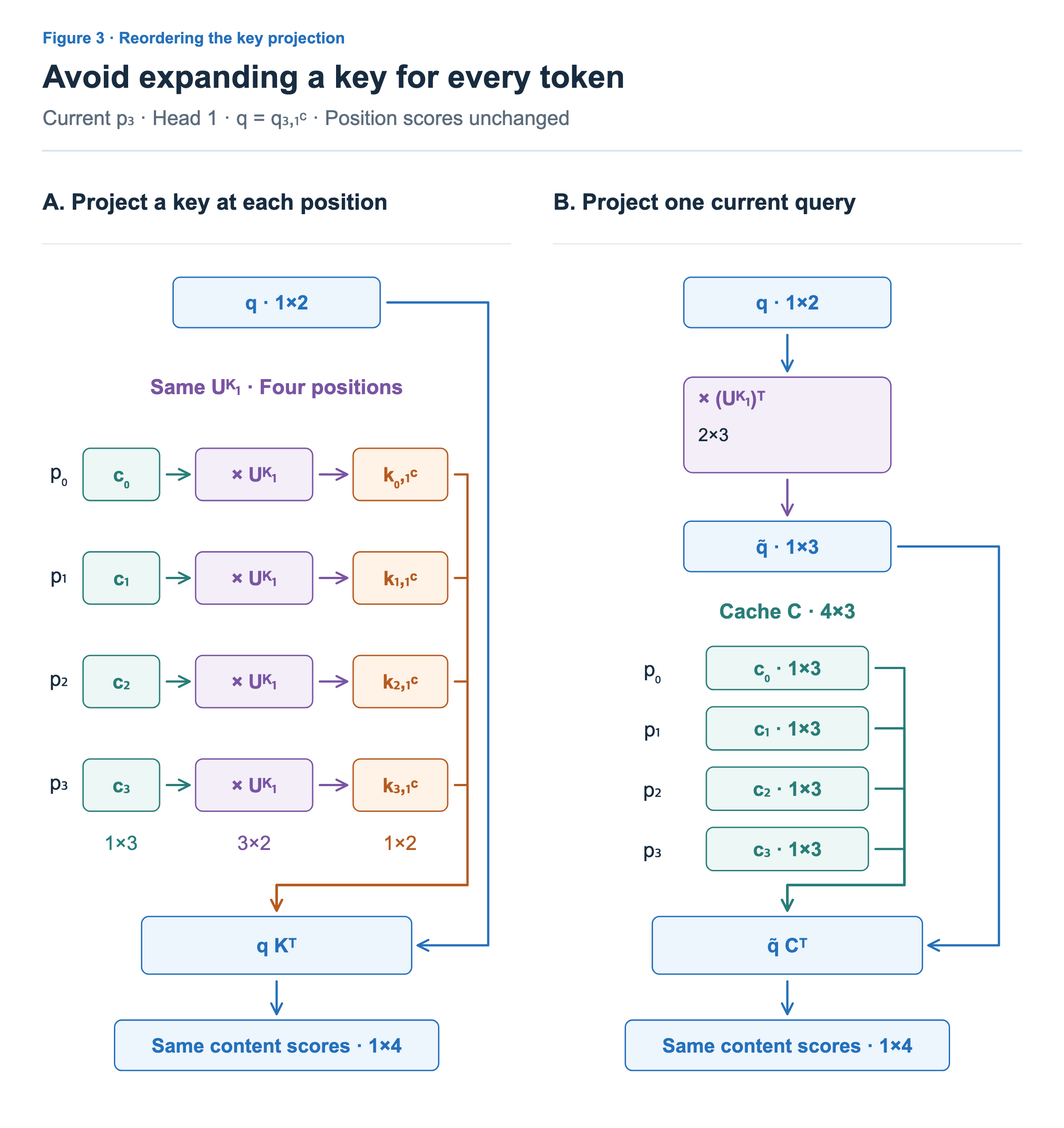
Write the current content query as for brevity. The content score at position is the dot product of and . With row vectors, we transpose the key side to form a dot product. The superscript T means exchanging rows and columns.
Compare what each side computes first. The left side multiplies the latent vector by to produce a key. The right side first multiplies the current query by the transposed projection. Call the result ; its shape is (1×2)×(2×3) = 1×3. We can now take its dot product directly with the 1×3 latent vector . This does not arbitrarily swap the order of factors. Transpose properties and the associativity of matrix multiplication let us regroup the computation.
Check this with small numbers. Suppose selects the first two components of = [1, 2, 3], as in the previous article. The content key is [1, 2], whose dot product with = [2, 1] is 2×1 + 1×2 = 4. Applying the transpose of that same projection to instead gives = [2, 1, 0]. Its dot product with is also 2×1 + 1×2 + 0×3 = 4.
The same relation holds at other positions. Let be the 4×3 matrix whose rows are the four latent vectors. Path A constructs four keys with and then computes scores. Path B constructs once for the current head, then computes directly with the four rows of .
Both results contain four content scores, with shape 1×4. Even as the cache grows, the current query’s transformation is not repeated for each position. Reading positions and computing scores with the transformed query still remain. The four projection blocks illustrate vector-level computations; they do not imply four separate GPU kernel launches.
Why the RoPE path is separate
We can now explain why the previous article cached positional keys separately. If we applied position ’s RoPE rotation to each expanded content key, the key projection would be followed by a rotation that varies by position. Moving this to the query side would make the query transformation depend on the position being read. We could no longer use one transformed query across all positions in the same way.
MLA applies RoPE to separate query/key parts, allowing the content path to keep the reordering in Figure 3. Positional scores are still computed separately and added as in Figure 2. DeepSeek-V2’s decoupled RoPE explanation
This does not mean latent vectors can never contain position-related information. The key question is which path receives explicit position-dependent rotation. Nor should we change the scaling divisor to √(3+2) because the content dot product now uses a three-dimensional latent space. It computes the same scores, so we retain √(2+2).
Moving the value projection after the weighted sum
Once we add the positional scores and apply softmax, we know how much to use each position. Collect these attention weights into row vector , of shape 1×4. These weights are input-dependent proportions, distinct from the learned projection matrices.
Both paths in Figure 4 start with the same cache and the same attention weights. A constructs a value at each position before taking their weighted sum. B takes a weighted sum of latent vectors first.
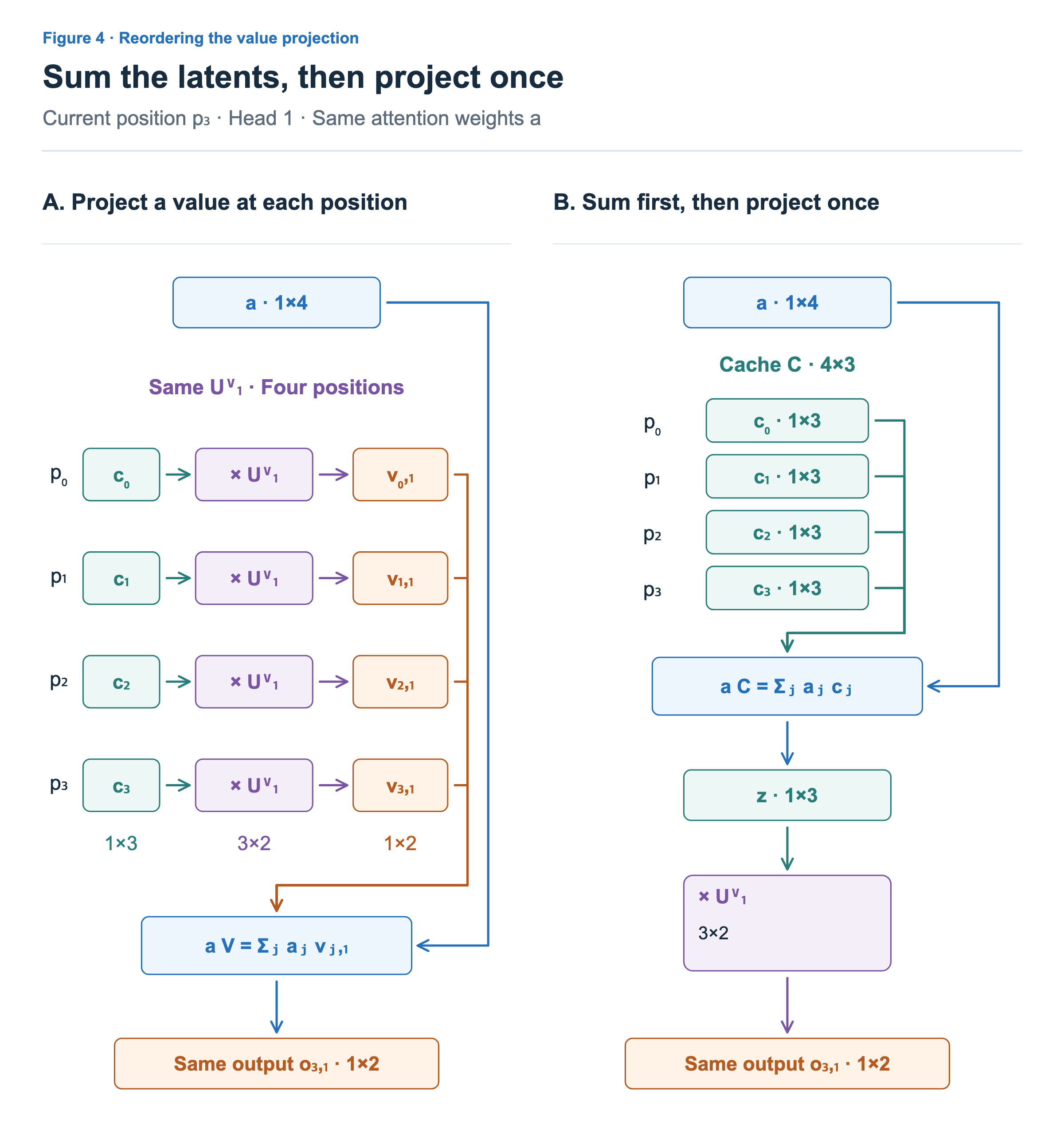
A applies the 3×2 projection to the 4×3 cache , producing a 4×2 value matrix. Multiplying by combines the four values into a 1×2 output. B first multiplies by , producing a 1×3 vector . Each component of combines that component across four positions using the same attention weights.
Applying to once therefore gives the same 1×2 output. For a linear transformation, applying the same projection at each position and then combining the results is equivalent to combining first and applying that projection afterward.
Assume the following latent vectors and attention weights. We retain = [1, 2, 3] from the earlier example; the other positions and weights are chosen to check the computation.
| Token position | Latent vector | Weight |
|---|---|---|
| [1, 0, 1] | 0.1 | |
| [0, 1, 1] | 0.2 | |
| [1, 1, 0] | 0.3 | |
| [1, 2, 3] | 0.4 |
As for head 1 in the previous article, let produce [first component + third component, second component]. A’s values are [2, 0], [1, 1], [1, 1], and [4, 2]. Their weighted sum using the table is [2.3, 1.3].
B combines the latent vectors first. The first component is 0.1×1 + 0.2×0 + 0.3×1 + 0.4×1 = 0.8. Computing the other components similarly gives = [0.8, 1.3, 1.5]. Applying gives [0.8 + 1.5, 1.3] = [2.3, 1.3], the same result.
Latent vectors are shared across heads, but the attention weights that combine them and the final value projection differ by head. Thus, and the final output are computed per-head. Also, we have not moved softmax across a projection. Scores and softmax still determine the weights; we only reorder the weighted sum with those weights and a linear projection.
Combining with query and output projections
Figure 3 moved the key projection to the query, and Figure 4 moved the value projection after the weighted sum. Precombining these moved projections with the existing query or output projection is called projection absorption. The two projections shown separately for clarity can be computed as one matrix multiplication during inference.
The associativity shown so far also holds at a given computation step during training. In inference, learned weights are fixed, so consecutive projection matrices can be multiplied in advance and reused across tokens.
On the query side, consider → → → transposed → . is 3×2 and transposed is 2×3, so pre-multiplying them gives a 3×3 matrix. Applying this composite matrix to produces directly, without separately constructing and then transforming the content query. The positional query path remains separate.
The value side extends similarly. Let denote head 1’s portion of the output projection that combines head outputs. Here, it maps a two-component head output into the model dimension of 8, so has shape 2×8. Pre-multiplying and gives a 3×8 matrix. Applying it to directly yields head 1’s 1×8 contribution to the model-dimensional output. Summing all heads’ contributions gives the full output projection result.
This projection absorption is described in DeepSeek-V2 §2.1.2. If the weights change, the composite matrix must be recomputed. If normalization or a nonlinear operation lies between projections, we cannot skip it to combine them. Reordering floating-point computations can also introduce small rounding differences.
Benefits and limits of reordering
Trace the work at the current again. We build queries from the current input and add its KV latent vector and positional key to the cache. Each head uses its transformed query to read the four latent rows, computes content scores, and adds positional scores. Softmax weights combine the latent vectors, followed by the value and output projections.
This computation does not need to materialize all expanded per-head past K and V vectors as intermediates. But reading past positions and computing attention scores and weighted sums still remain. A longer context still adds cache rows.
A smaller stored representation does not make every computation lower-dimensional. The expanded content keys and values in our example are two-dimensional, while latents are three-dimensional. After reordering, content dot products and weighted sums operate on three-dimensional rather than two-dimensional vectors. We therefore need to consider changes in dot-product and weighted-sum computation alongside savings in KV reconstruction and memory use.
Actual runtime depends on context length, the number of requests, dimensions, kernels, and hardware. Prefill, which processes multiple queries together, need not choose the same computation path as decode, which processes one current query. The actual speedup from reordering must therefore be measured for the model and environment in use.
The previous article examined what to cache; this article examined how to compute attention from that cache. A shared latent representation reduces the cache, and reordering lets attention read it directly. Next, we will go beyond reading every position’s representation and explore structures that restrict the range and choice of tokens attention reads.