Local and Sparse Attention: Reading Fewer Token Positions

The previous article changed how KV is represented and how its computation is ordered. This time, we will reduce the range of tokens each query reads. Sparse Attention applies attention to only some positions, rather than every past position. Sliding Window Attention (SWA), which reads only nearby positions, is one form of sparse attention.

We will first examine how SWA determines which positions to read, then extend it to patterns that also read selected distant positions. Next, we will trace how information travels through multiple layers and examine when reducing the positions read also allows a smaller KV cache. This article covers connection rules determined by position, independently of token content.

Reading nearby positions with SWA

Suppose we have eight tokens, $p_{0}$ through $p_{7}$ , and are processing $p_{7}$ . For one query head in one attention layer, ordinary causal attention computes scores against keys at all eight positions from $p_{0}$ through $p_{7}$ and takes a weighted sum of their values. Here, causal means that future positions cannot be read. The figures label this pattern, which reads the current position and every past position, Full causal.

SWA adds a distance limit. In this article, a window of 3 means the current position and the two immediately preceding positions: three in total. At $p_{7}$ , it reads only $p_{5}$ , $p_{6}$ , and $p_{7}$ . At the next position, $p_{8}$ , the range moves to $p_{6}$ , $p_{7}$ , and $p_{8}$ . It is called a sliding window because the range moves with the current position.

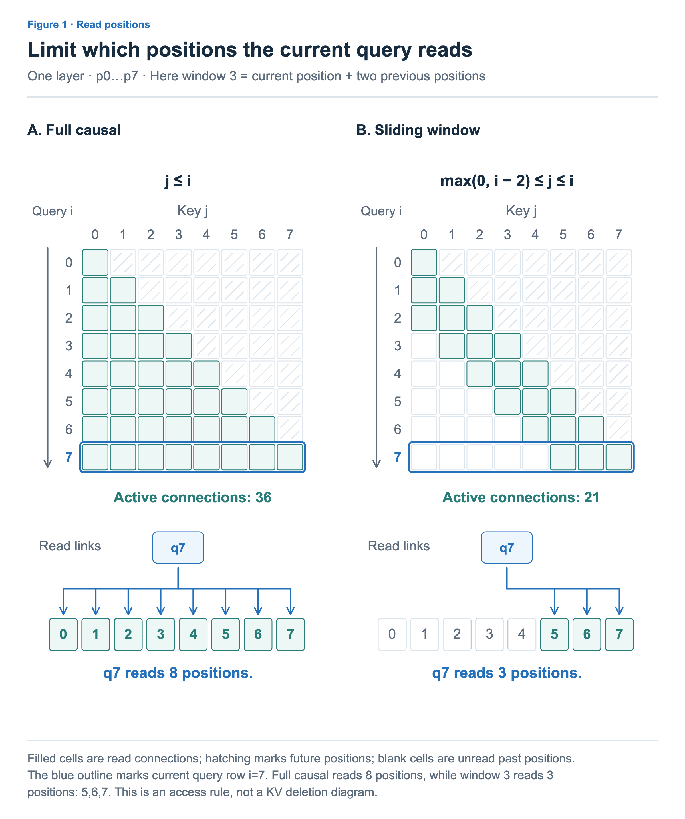
Two grids with query position as rows and key position as columns compare full causal attention and a window of 3. Position 7 reads all eight positions or positions 5, 6, and 7. The total connection counts are 36 and 21.

In Figure 1, the vertical axis is the query’s token position, and the horizontal axis is the key’s token position. Neither axis represents heads or vector components. Filled cells in a row indicate the positions that query reads; their shading does not represent attention weights. In the last row, outlined in blue, full causal attention reads eight cells, while SWA reads three.

Once the positions are selected, the computation is familiar attention. We compute scores between $q_{7}$ and the three selected keys, apply softmax over those three positions, and take a weighted sum of their values. Excluded positions do not participate in this weighted sum. With a mask, their scores receive negative infinity before softmax, giving them zero weight. Simply setting their scores to zero is a different computation: they would still receive positive weights after softmax.

What is fixed here is the rule for which positions are connected. The attention scores and weights at selected positions still vary with the content of the query and keys. SWA is also not a reordering of computation that preserves the output of full attention. Restricting which information can be read can change the output.

The full grids show the connections used when processing all eight tokens. Full causal attention has 1 + 2 + … + 8 = 36 connections, while a window of 3 has 1 + 2 + 3 + 3 + 3 + 3 + 3 + 3 = 21. The comparison of 8 versus 3 for the current $p_{7}$ alone is different from 36 versus 21 across all eight tokens. With a fixed window, the number of positions one query reads remains bounded even as the context grows.

The architecture section of the Mistral 7B paper gives a real model example using SWA. Papers and implementations can differ in how they count window boundaries, so we retain the definition used in these figures: three cells including the current position.

Reading nearby and distant positions together

With SWA, a token sufficiently far from the current position cannot be read directly. One way to address this is to add connections to designated distant positions alongside the nearby connections. A sparse attention pattern does not have to be one contiguous window.

Figure 2 compares two rules. The left adds the first position, $p_{0}$ , to the latest three positions. The right adds positions spaced four positions apart, such as $p_{0}$ and $p_{4}$ , to the latest three. Both are educational examples illustrating different connection rules, rather than reproductions of a particular model architecture.

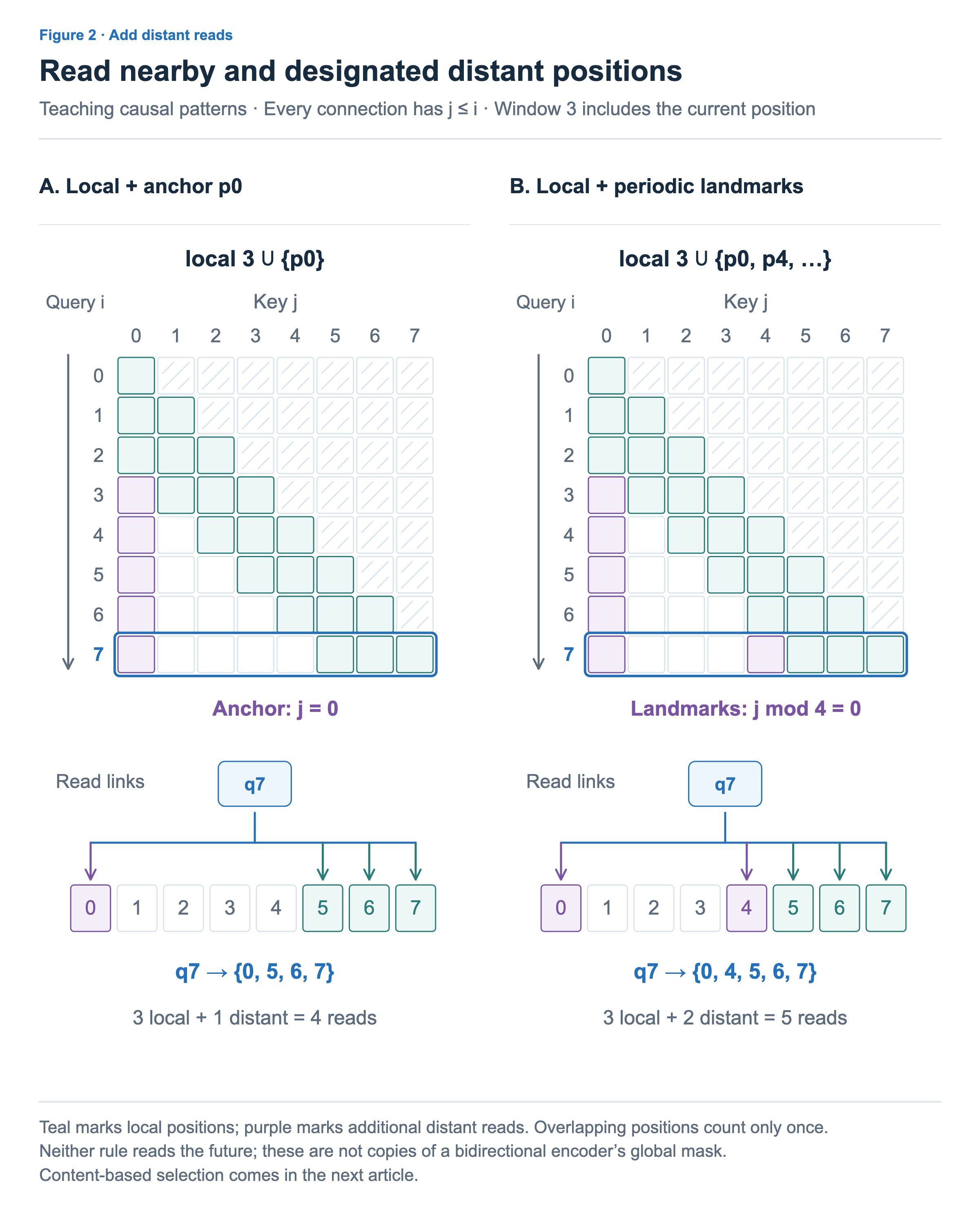
Two rules add the first position or positions spaced four apart to the latest three positions. At position 7, the read sets are 0, 5, 6, 7 and 0, 4, 5, 6, 7.

On the left, the current $q_{7}$ reads $p_{0}$ as well as $p_{5}$ , $p_{6}$ , and $p_{7}$ . The anchor in the figure is a designated position that remains available to read. The direct connection to information at the first position is retained, but this does not make every intervening position readable. Positions $p_{1}$ through $p_{4}$ are still excluded.

On the right, landmarks are positions designated at regular intervals. The positions read by $q_{7}$ are $p_{0}$ , $p_{4}$ , $p_{5}$ , $p_{6}$ , and $p_{7}$ : five in total. When processing $p_{4}$ , that position belongs to both the window and the designated set, but is read only once. Both rules exclude future positions, so $p_{3}$ cannot read $p_{4}$ , which is still in the future.

Adding the first position contributes only one extra position once the window has moved far enough. In contrast, adding every regularly spaced position includes more positions as the context grows. Thus, a fixed rule does not necessarily imply a fixed number of positions read per query. The computation depends on the spacing and the number of positions retained.

Longformer also proposes an architecture combining local and global connections. Figure 2, however, is a causal example that cannot read the future; it does not reproduce Longformer’s bidirectional connections. The key idea here is that connections to nearby positions and selected distant positions can be designed together.

Information flowing through multiple layers

In pure SWA, with no direct connections to distant positions, can information outside the window travel at all? The range read directly by one layer differs from the range of inputs that can influence a representation after several layers. A vector from the previous layer can already contain information from other positions that layer read.

Return to the example in which every attention layer uses a window of 3. In Figure 3, the horizontal axis is token position, and the vertical axis is model depth. L0 denotes the input, while L1 through L3 denote representations after each layer. Moving upward means advancing to the next model layer, not advancing time to generate a new token.

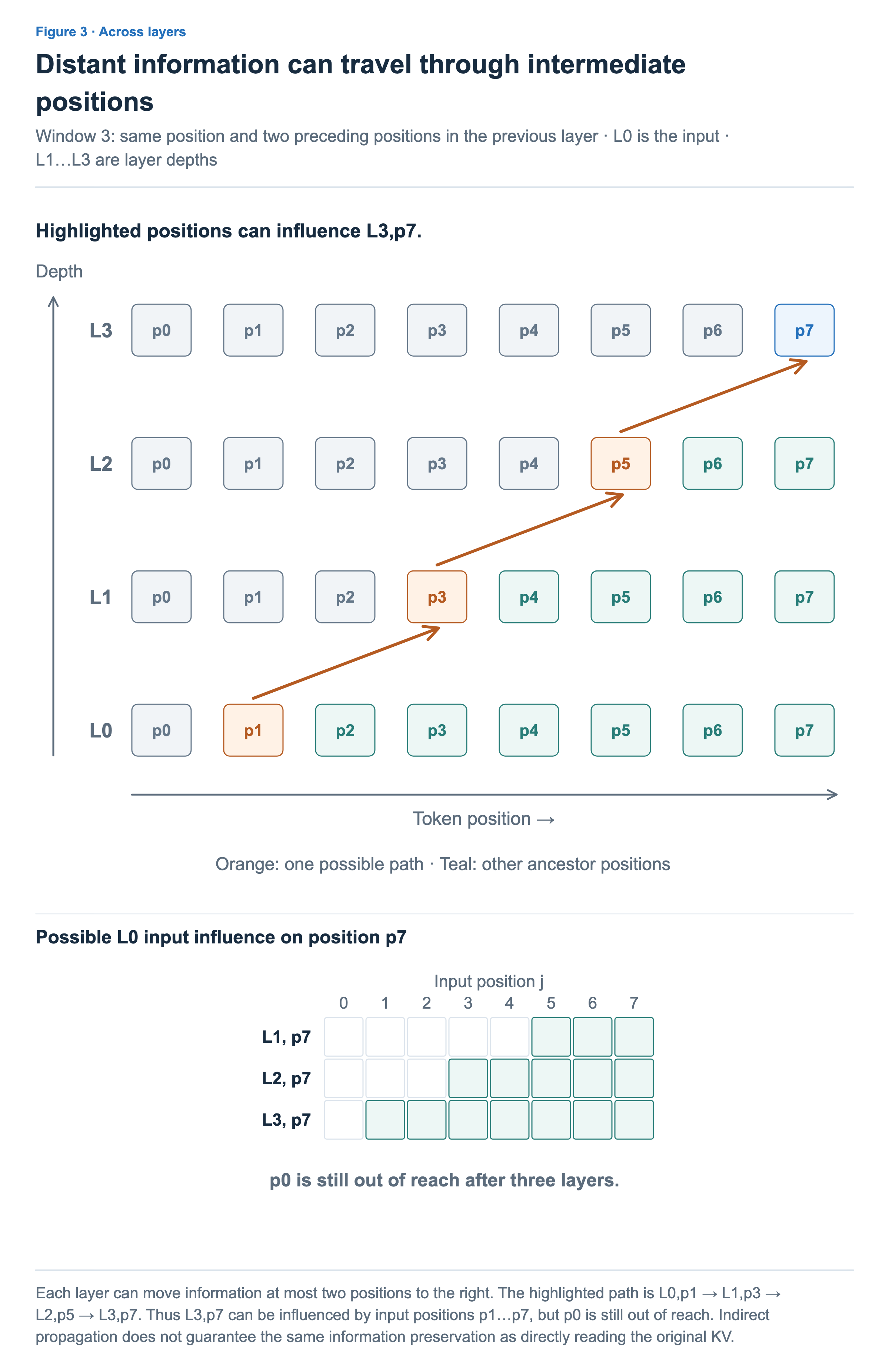
Token positions and layer depth are separate axes. Information from input position 1 can pass through first-layer position 3 and second-layer position 5 to third-layer position 7. Its input receptive field spans positions 1 through 7.

At L1, $p_{7}$ reads $p_{5}$ , $p_{6}$ , and $p_{7}$ from L0. At L2, $p_{7}$ still reads only $p_{5}$ , $p_{6}$ , and $p_{7}$ from the layer immediately below, but L1’s $p_{5}$ can already reflect information from L0’s $p_{3}$ , $p_{4}$ , and $p_{5}$ . Tracing these paths expands the input range that can influence L2’s $p_{7}$ to $p_{3}$ through $p_{7}$ . At L3, it expands to $p_{1}$ through $p_{7}$ .

The orange arrows show one path from the farthest position: input $p_{1}$ → first-layer $p_{3}$ → second-layer $p_{5}$ → third-layer $p_{7}$ . Information can move forward by at most two positions per layer, so three layers can connect an input up to six positions away. Position $p_{0}$ is seven positions away from $p_{7}$ and cannot yet reach it through the three layers in this example.

This connected range is often called the receptive field. However, the existence of a path does not mean all information within that range is preserved intact. Information from multiple positions is mixed and transformed in intermediate vectors; this differs from the current query reading the original KV at a distant position directly. Stacking layers broadens the range of influence, but does not guarantee the same output as full attention.

Read range and cache storage

If we read fewer positions, can we delete the rest from the KV cache? The deciding factor is whether a position can be read again later, not whether it was read now.

The left side of Figure 4 shows a layer that never rereads positions once they leave its window. At $p_{7}$ , it needs KV for $p_{5}$ , $p_{6}$ , and $p_{7}$ ; at $p_{8}$ , it needs $p_{6}$ , $p_{7}$ , and $p_{8}$ . Position $p_{5}$ will never reenter this layer’s window, so its KV can be discarded after processing $p_{7}$ .

A window-only layer discards KV for position 5 and adds position 8 when moving from position 7 to 8, retaining the latest three positions. A separate full-attention layer retains its own KV. A layer where future queries may select other positions keeps eight positions even while reading only three.

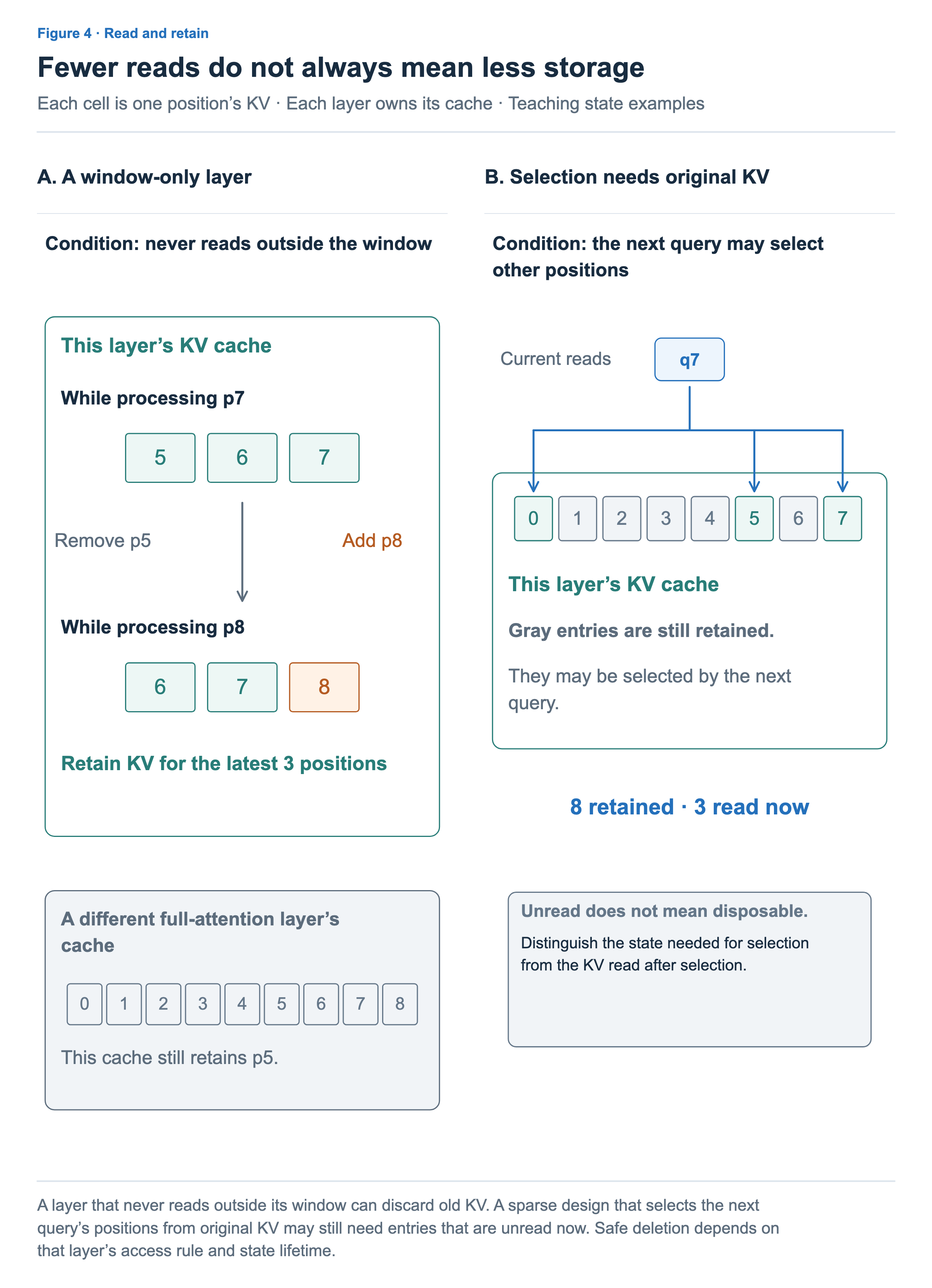
By replacing old KV as new positions are added, this layer can keep a cache sized for the latest three positions. In physical memory, existing slots can be overwritten in a circular fashion. The figure shows states during token-by-token processing; it does not depict intermediate buffers used when processing multiple tokens together.

Caches must be distinguished by layer. If another layer in the same model uses full attention, a future query can read $p_{5}$ again, so that layer must retain its own KV for $p_{5}$ . Being able to delete a position in an SWA layer does not imply deleting its KV from other layers as well.

The right side shows a case where the current query selects only some positions, but the next query may select different ones. Although $q_{7}$ currently reads only $p_{0}$ , $p_{5}$ , and $p_{7}$ , this example requires the original KV for selection, so the other positions are retained too. Three positions are read, while eight remain in the cache. The next article will examine the details of content-based position selection.

The fixed patterns in Figure 2 also require storage that matches their rules. If the first position is always read, its KV must remain after $p_{0}$ leaves the window. If regularly spaced positions continue to be read, they must remain too. The name sparse attention alone does not determine the cache size.

What changes when connections are reduced

This article changed the positions a query reads, rather than the size of each KV vector. SWA restricts reads to nearby positions, while other fixed patterns add selected distant positions. Through multiple layers, information can arrive from a wider input range than one layer’s window, but this is not equivalent to retaining every direct connection.

An implementation that actually computes only selected connections can reduce the operations needed for attention scores and the weighted sum of values. Conversely, computing every score and then applying a mask does not skip that computation merely because the connections are sparse. Execution speed also depends on how efficiently the kernel handles the chosen pattern.

When reading an architecture, therefore, check which positions are read, how their count grows with context length, and how much KV must remain for later reads. The next article moves from positions designated in advance to an indexer that selects positions based on the current query and token content.