Sparse Attention Indexers: Choosing Positions by Content

The previous article limited the read range using fixed rules, such as nearby positions or positions at regular intervals. But the information the current token needs may lie outside that range. Even a distant position should be directly accessible if it matters to the current computation.

This article introduces an indexer that compares the current input with the content at each position to choose which positions to read. We will first trace how an index query and index keys select positions for the main attention computation. Then we will examine how selection changes as tokens are processed one at a time and how it can be combined with a window of recent positions.

Selecting positions with an index query and keys

If we compute main attention scores against every key and only then keep a subset, we have already paid the cost of computing all those scores. The purpose of an indexer is to narrow the candidates first with a lighter computation than main attention. It uses separate query and key representations for position selection.

Figure 1 selects three of eight positions at the current position $p_{7}$ . Labels $p_{0}$ through $p_{7}$ denote token positions, not head numbers. $h_{7}$ is the current token vector entering this attention layer. The index query and the main attention query are derived from the same input, but use different projections.

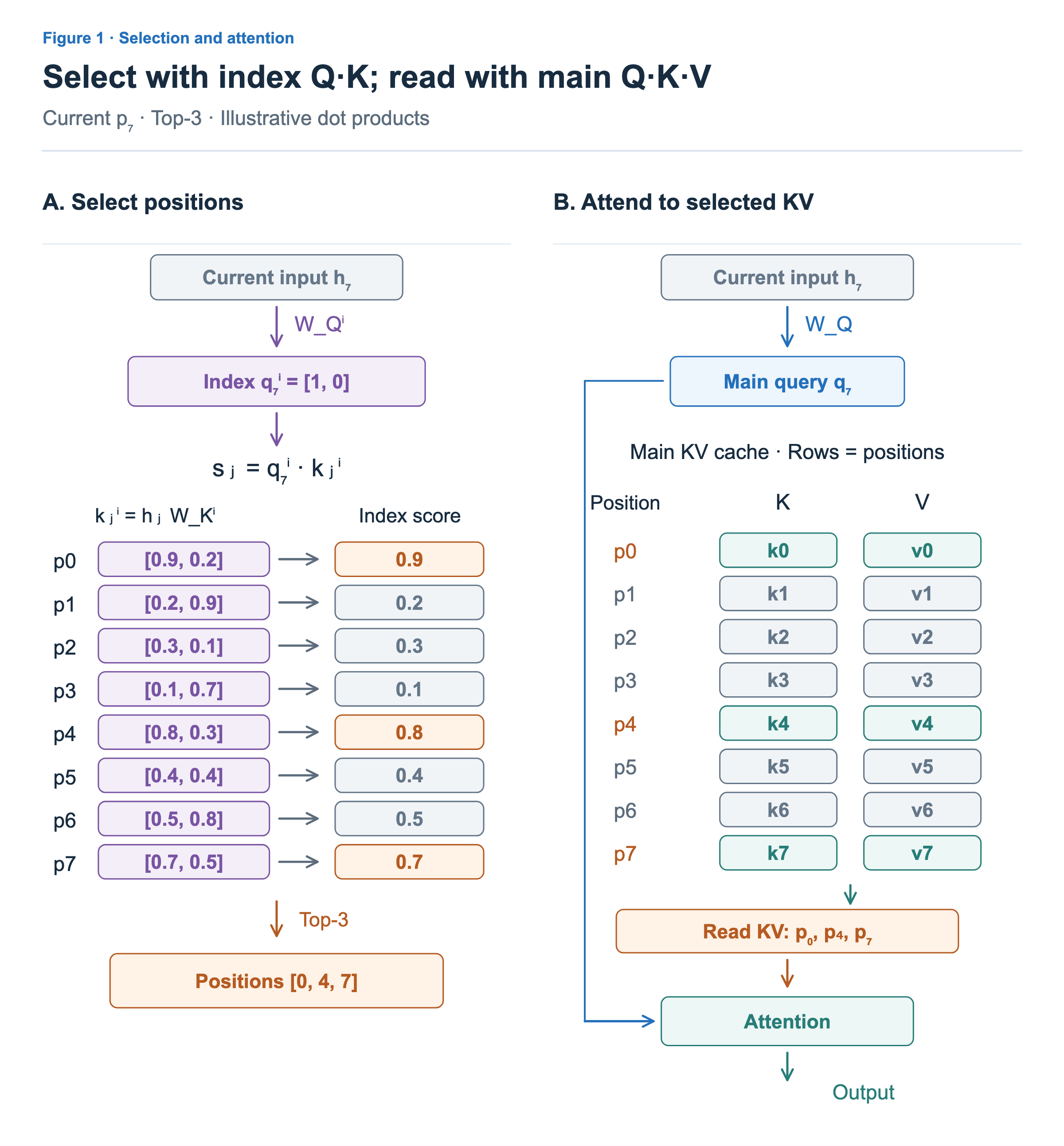
Separate projections produce an index query and a main query. Dot products with per-position index keys select positions 0,4,7. Main attention reads its own keys and values at those positions.

On the left, $q_{7}^{i}$ and $k_{j}^{i}$ are the index query and index key, respectively. The superscript i marks the indexer representations; the subscript denotes a token position. The example uses two-component vectors to make the arithmetic easy to follow. The index query is [1, 0], and the index key at position 0 is [0.9, 0.2]. Their dot product is 1 × 0.9 + 0 × 0.2 = 0.9.

Applying the same calculation to all eight positions gives selection scores of [0.9, 0.2, 0.3, 0.1, 0.8, 0.4, 0.5, 0.7], in position order. The three largest are 0.9 at position 0, 0.8 at position 4, and 0.7 at position 7, so Top-3 selects positions 0, 4, and 7. Top-k means choosing the k highest-scoring candidates.

On the right, we read the main attention keys and values at these three positions. The main query $q_{7}$ and the selected keys produce attention scores, and softmax weights over the selected positions are used to combine their values. This is the same attention computation we have already learned. The difference is that the participating positions are chosen first.

The selection scores 0.9, 0.8, and 0.7 are not used directly as weights on the values. The indexer returns positions to read; main attention separately determines how much to incorporate the information at those positions. Index keys do not replace the main attention keys either.

In the official DeepSeek-V3.2 implementation, the indexer also computes scores using separate query and key representations and returns selected positions. The actual implementation uses multiple indexer heads and positional information, so the two-component dot product in the figure does not reproduce the full computation. The figure separates the role of choosing positions from the role of reading the selected KV. The representation used to store main KV can also vary, as in the MLA we studied earlier.

Selection can change as generation proceeds

Do the selected positions remain fixed afterward? Consider processing $p_{6}$ and then $p_{7}$ in the same layer. Previously computed index keys and main KV are retained, but the query derived from the current input changes. The new position’s keys and KV are also added to the caches.

At p6, q6=[0,1] scores positions0–6 and selects1,3,6. After adding p7 keys and KV, q7=[1,0] scores positions0–7 and selects0,4,7. Future position7 is absent from p6 candidates.

When processing $p_{6}$ , only positions 0 through 6 are candidates. Position 7 is still in the future and is excluded. The index query $q_{6}^{i}$ is [0, 1], so the second component of each index key becomes its score. The scores are [0.2, 0.9, 0.1, 0.7, 0.3, 0.4, 0.8], selecting positions 1, 3, and 6.

When processing $p_{7}$ next, we add its index key and main KV. The index query $q_{7}^{i}$ is now [1, 0], so scores come from the first components. The selected positions are 0, 4, and 7, as in Figure 1. Even with unchanged past keys, a different current query assigns different scores to the same past positions. Selection can change during actual generation too, although it does not have to change at every step.

This example also illustrates the distinction between the read range and cache storage from the previous article. Positions 0 and 4, which were not read at $p_{6}$ , are read at $p_{7}$ . Discarding all KV outside the Top-3 at $p_{6}$ would prevent that subsequent selection from being used.

At $p_{7}$ , the figure reads main KV at just three positions, but the cache retains all eight. As long as the indexer can consider any past position again, its index key and the main KV that may be read again must remain available. Selecting fewer positions to read does not by itself reduce cache storage in the same proportion.

Combining selected positions with a recent window

Selecting only the highest-scoring positions can leave recent positions out. In Figure 1, positions 5 and 6, immediately before the current position, are not in the Top-3. To always read the nearby context, we can add a sliding window to the indexer’s selection.

As in the previous article, a window of 3 includes the current position and the two immediately preceding positions. At $p_{7}$ , these are positions 5, 6, and 7. Figure 3 combines this window with positions 0, 4, and 7 selected by the indexer.

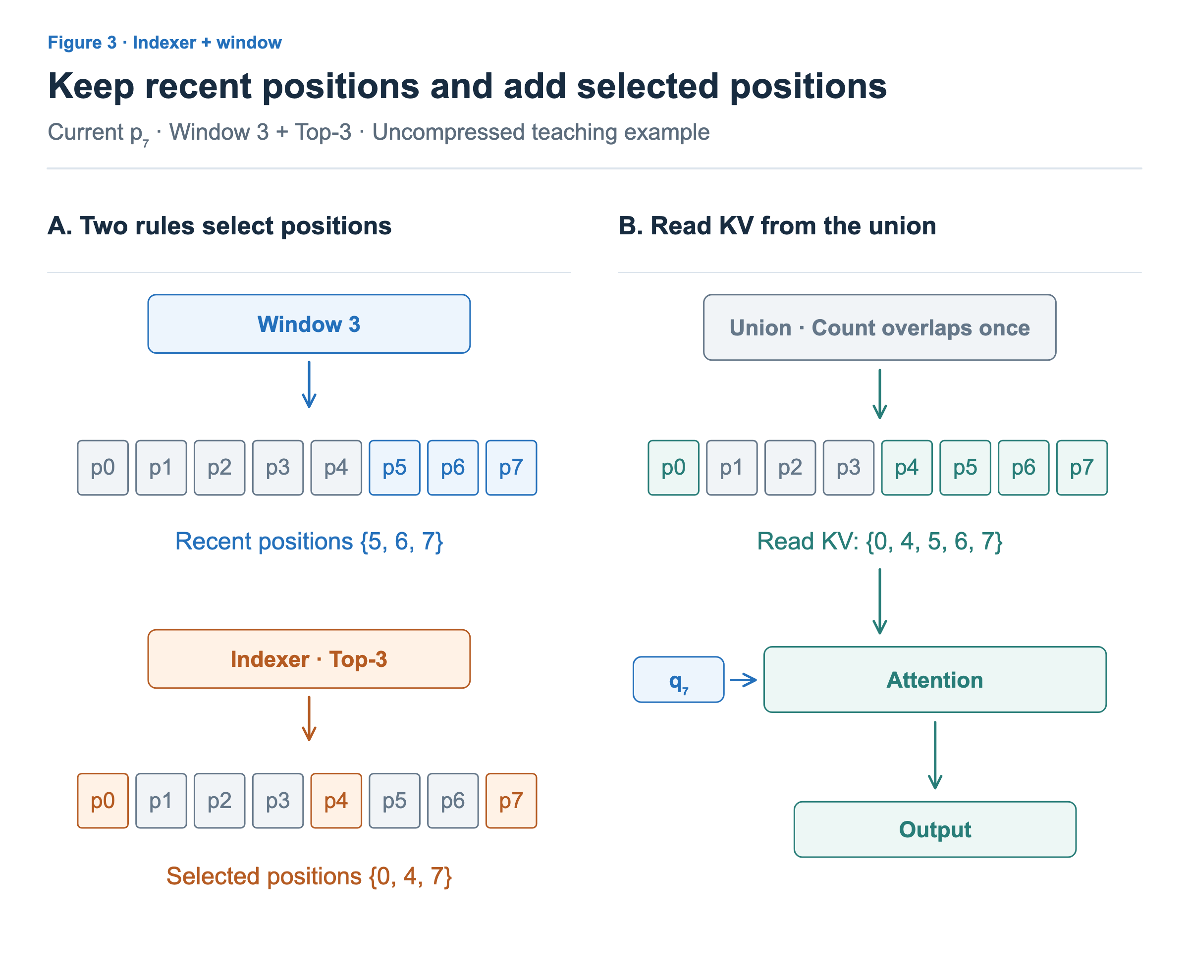
At position7, the window includes5,6,7 and the indexer selects0,4,7. Original KV at0,4,5,6,7 enters main attention with the query, counting overlapping7 once.

The union contains positions 0, 4, 5, 6, and 7. Position 7 appears in both sets, but it refers to the same original KV and is read only once. Main attention is computed over these five positions together. The window ensures that the three recent positions are included, while the indexer provides content-dependent access to other positions.

In this figure, positions inside the window are also indexer candidates. Thus, a window of 3 plus Top-3 results in five positions read, not six. Another possible design excludes the window from the candidate set and selects k additional positions outside it. With enough candidates, that design spends the entire selection budget of k on positions outside the window. Combining a window with an indexer does not, by itself, specify the candidate range or how overlaps are handled.

Selection cost and reading cost

The indexer reduces the positions read by main attention but adds computation for selection. Even in Figure 1, main attention reads three positions while the indexer compares index keys at eight positions. As the context grows, reading candidate keys, computing scores, and finding the Top-k also become more expensive.

The combination is beneficial when the cost saved in main attention exceeds the added selection cost. The outcome depends on the size of the index representations, the number of indexer heads, the number of selected positions, how selected KV is fetched, and the kernel implementation. Reading three of eight positions does not mean total execution time falls to 3/8.

Selection accuracy matters too. If the indexer misses a position that main attention would rely on, its value cannot contribute directly to this output. Selecting more positions allows more information to be read, but also increases cost. An indexer is a model design that limits the information read, rather than a rearrangement of computation guaranteed to preserve the result of attention over all positions.