Token-Axis Compression: Reading Summaries of Multiple KV Positions

The previous article used an indexer to choose KV positions to read. This time, we will examine how information from several token positions is combined into a single summary KV entry before selection. Reading entries that represent several positions, rather than one entry per position, lets us handle a long context with fewer entries.

We will first distinguish the compression axis from the one we learned about in MLA. Then we will trace the calculation that turns two input positions into one summary vector, examine why completed summaries are read alongside recent per-token KV, and finally connect compression to selecting summaries with an indexer.

Vector width and the number of token positions

Saying that KV storage shrinks does not tell us what becomes smaller. When per-position vectors are stacked as rows, reducing the number of components in each row and combining several rows into one are different changes.

Both sides of Figure 1 start with eight rows and four components. Rows denote token positions $p_0$ through $p_7$, and columns denote vector components. The grid does not represent the number of heads.

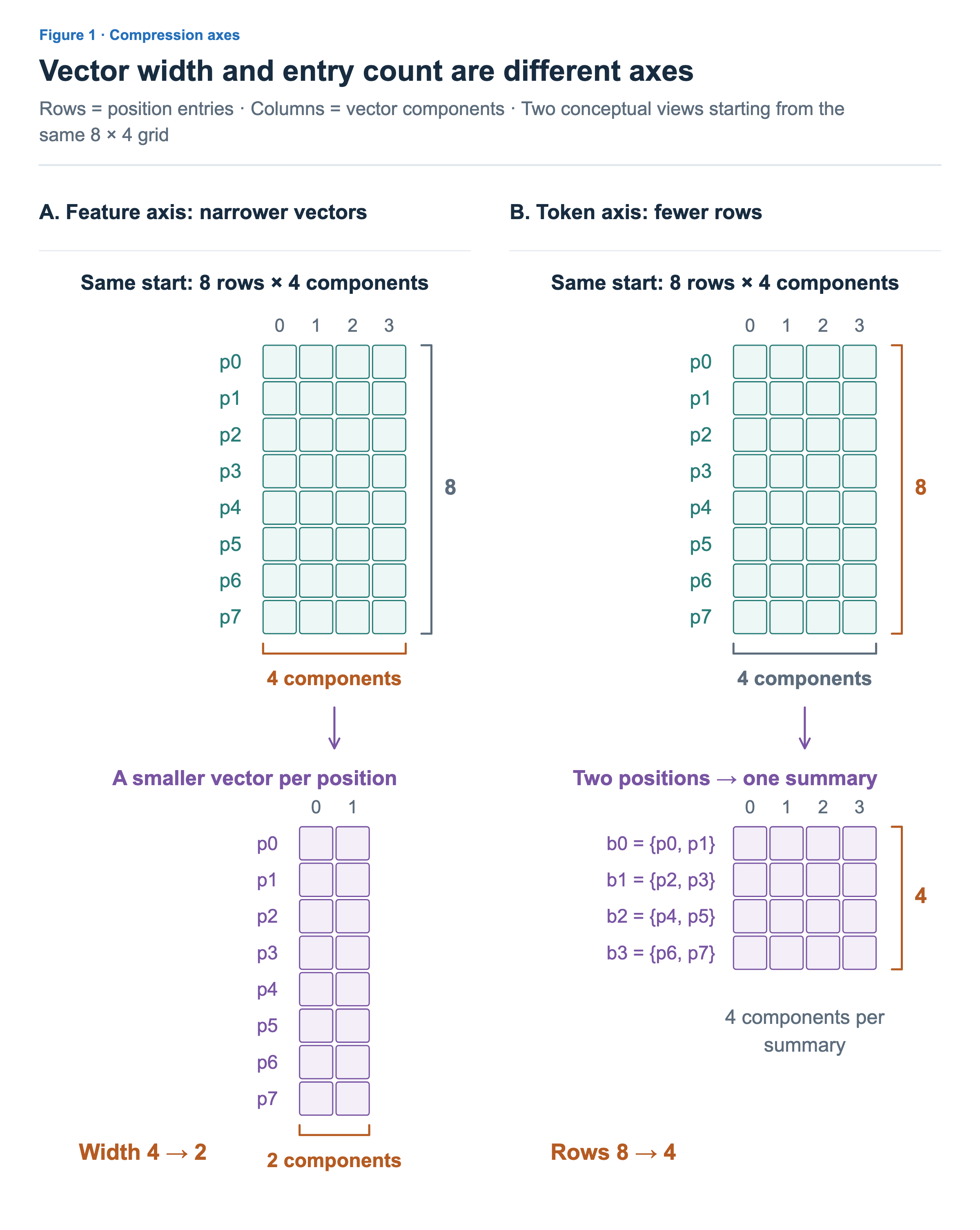
On the left, each position’s representation shrinks from four components to two. There are still eight positions, so the result has eight rows and two components. The latent representation in MLA’s storage structure can also be understood as reducing the width of the vector stored at each position. Actual MLA also has separate positional components, however, so this grid does not represent its entire cache size.

On the right, two adjacent positions form one summary. Positions $p_0$ and $p_1$ become $b_0$, while $p_2$ and $p_3$ become $b_1$. Each summary retains four components, while the number of entries falls from eight to four, giving four rows and four components. This is the token-axis compression covered in this article. Reducing the token count here means reducing the number of KV entries attention reads, not the number of output tokens the model generates.

Summary $b_0$ is not simply the original KV at $p_0$ left in place. It is a new representation that combines information from two positions. This also distinguishes compression from an indexer that selects positions: an indexer chooses some candidates, whereas compression combines information from several candidates into a new entry. The two final grids have the same number of cells, but that does not mean they contain the same information or involve the same computation.

Building a summary vector with two projections

We could simply average every component across two positions. Here, instead, we examine a learned way to determine how much each position contributes to each component. The same input feeds two paths. The content projection creates vectors to include in the summary, and the score projection creates scores used to determine how to mix that content.

The inputs in Figure 2 are the vectors $h_0$ = [1, 0] and $h_1$ = [0, 1] at two positions. Let H be the matrix that stacks them as rows. This example combines two positions into one while retaining two components.

The first step multiplies H by two different projection matrices, $W_u$ and $W_s$. These are learned parameters: $W_u$ produces content vectors, and $W_s$ produces per-component scores. The model learns the projection matrices; the projection outputs depend on the input. The matrix values in the figure are educational examples chosen to make the arithmetic easy to follow.

The two rows of the content projection $W_u$ are [2, 0] and [0, 4]. Multiplying $h_0$ by this matrix gives [2, 0], and multiplying $h_1$ gives [0, 4]. Stacking those results as rows gives the content matrix U. No positions have been combined yet: the content at each position has only been transformed.

The two rows of the score projection $W_s$ are [ln 3, 0] and [0, ln 3]. Multiplying the same input H by this matrix gives a score matrix S with those same values. The projection matrix and its output look identical here because we chose the identity matrix as the input; this is not true for a general input. The values ln 3 and 0 are not calculated from the content vector [2, 0]. They come from projecting the same input with a separate score matrix.

These scores are not used directly as weights. For each component, softmax is applied across the two positions. This normalizes each column vertically in the figure. For the first component, the scores [ln 3, 0] exponentiate to [3, 1]. Dividing by their sum, 4, gives [0.75, 0.25]. For the second component, the scores [0, ln 3] give weights [0.25, 0.75]. We chose ln 3 and 0 to obtain these simple proportions.

Each column of the resulting weight matrix A sums to 1. The first component takes 75% from position 0 and 25% from position 1; the second component does the reverse. The mixing proportions are set separately for each component, rather than applying one pair of proportions to the entire vector.

The second step multiplies corresponding components of U and A, then sums across positions. Unlike the earlier projection, this is elementwise multiplication, not matrix multiplication. The first component is 2 × 0.75 + 0 × 0.25 = 1.5, and the second is 0 × 0.25 + 4 × 0.75 = 3. The final summary $c_0$ is [1.5, 3]. Two per-position entries have become one summary while retaining two components.

These weights have a different role from the weights obtained by comparing the current query and keys in main attention. Compression weights build a summary; attention weights read the completed summaries. The current query does not participate in summary creation in Figure 2. Completed summaries can be cached and reused by later queries.

The Compressor in DeepSeek-V4’s official implementation likewise applies content and score projections to the same input, then compresses with a softmax and weighted sum over positions. The figure isolates that calculation in a small example. It omits the implementation’s positional bias, overlapping compression ranges, subsequent normalization, and positional processing. It does not mean that combining arbitrary existing KV entries this way preserves the original attention output exactly.

Completed summaries and recent per-token KV

To combine positions, their inputs must all have arrived. When processing tokens one at a time, some groups remain incomplete. At the same time, recent context can be retained as individual positions instead of relying entirely on summaries.

Figure 3 creates one summary for every two positions and separately retains KV for the latest three positions, including the current one. We will call this recent per-token KV. It means KV entries that have not been combined across positions, not the input vectors entering the model. “Original” in the figure likewise refers to entries before token-axis compression.

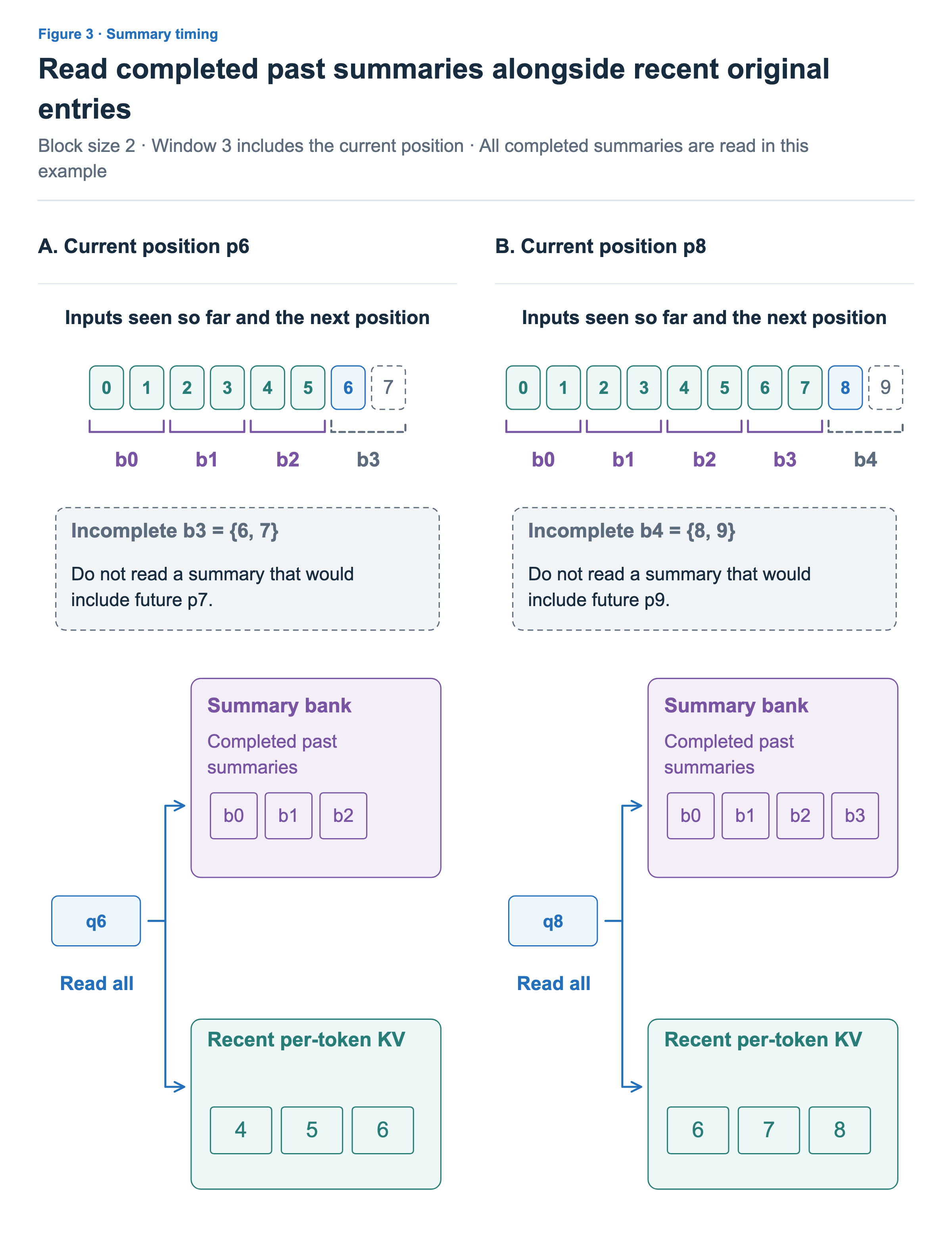
When processing $p_6$, summaries $b_0$ for $p_0$ and $p_1$, $b_1$ for $p_2$ and $p_3$, and $b_2$ for $p_4$ and $p_5$ are complete. But group $b_3$, which combines $p_6$ and $p_7$, cannot yet be completed. If $q_6$ read a summary containing future position $p_7$, it would be using future information.

Thus, $q_6$ reads completed summaries $b_0$, $b_1$, and $b_2$ alongside recent per-token KV at $p_4$, $p_5$, and $p_6$. The “Summary bank” in the figure is the cache of completed summaries. We temporarily leave selection aside and assume all completed summaries are read. Information at the current position $p_6$, which is not yet part of a summary, is available through recent per-token KV.

Why retain individual KV for $p_4$ and $p_5$ when they have already been combined into $b_2$? Summary $b_2$ is a single entry mixing two positions. A query can assign a weight to $b_2$, but it cannot separate $p_4$ and $p_5$ within it and assign different attention weights to each. Keeping recent per-token KV lets attention distinguish and read nearby positions individually.

Summary creation and recent KV retention follow separate rules. A summary is added when its group is complete, while individual KV remains as long as it is within the window. Compression therefore does not immediately delete individual KV for those positions. Summary $b_2$ and positions $p_4$ and $p_5$ contain information from the same period, but they are different read entries. This differs from the previous article’s case where a window and an indexer selected the same original position and the duplicate was removed.

On the right, processing has reached $p_8$, so summary $b_3$ for $p_6$ and $p_7$ is also complete. Recent per-token KV now covers $p_6$, $p_7$, and $p_8$. Positions $p_4$ and $p_5$ have left the recent window, so their individual KV is removed from this path, while their information remains summarized in $b_2$. Summary $b_4$, which would include the still-future position $p_9$, is not read.

Summarizing every two positions does not make this cache fixed in size. Recent per-token KV stays at three entries, but one past summary is added for every two input positions. There is also intermediate state needed while building summaries. Token-axis compression slows the growth in the number of entries storing past information; it does not turn an entire long context into a single fixed-size state.

Combining compression and an indexer

As summaries accumulate, we can choose to read only some of them. Whereas the previous article’s indexer selected token positions, it now selects compressed summary entries. Another design is to create sufficiently few summaries and read them all.

Figure 4 shows two paths for handling completed past positions $p_0$ through $p_{15}$ at the current position $p_{16}$. Both also read recent per-token KV at $p_{14}$, $p_{15}$, and $p_{16}$. What changes is the group size for past positions and how summaries are selected.

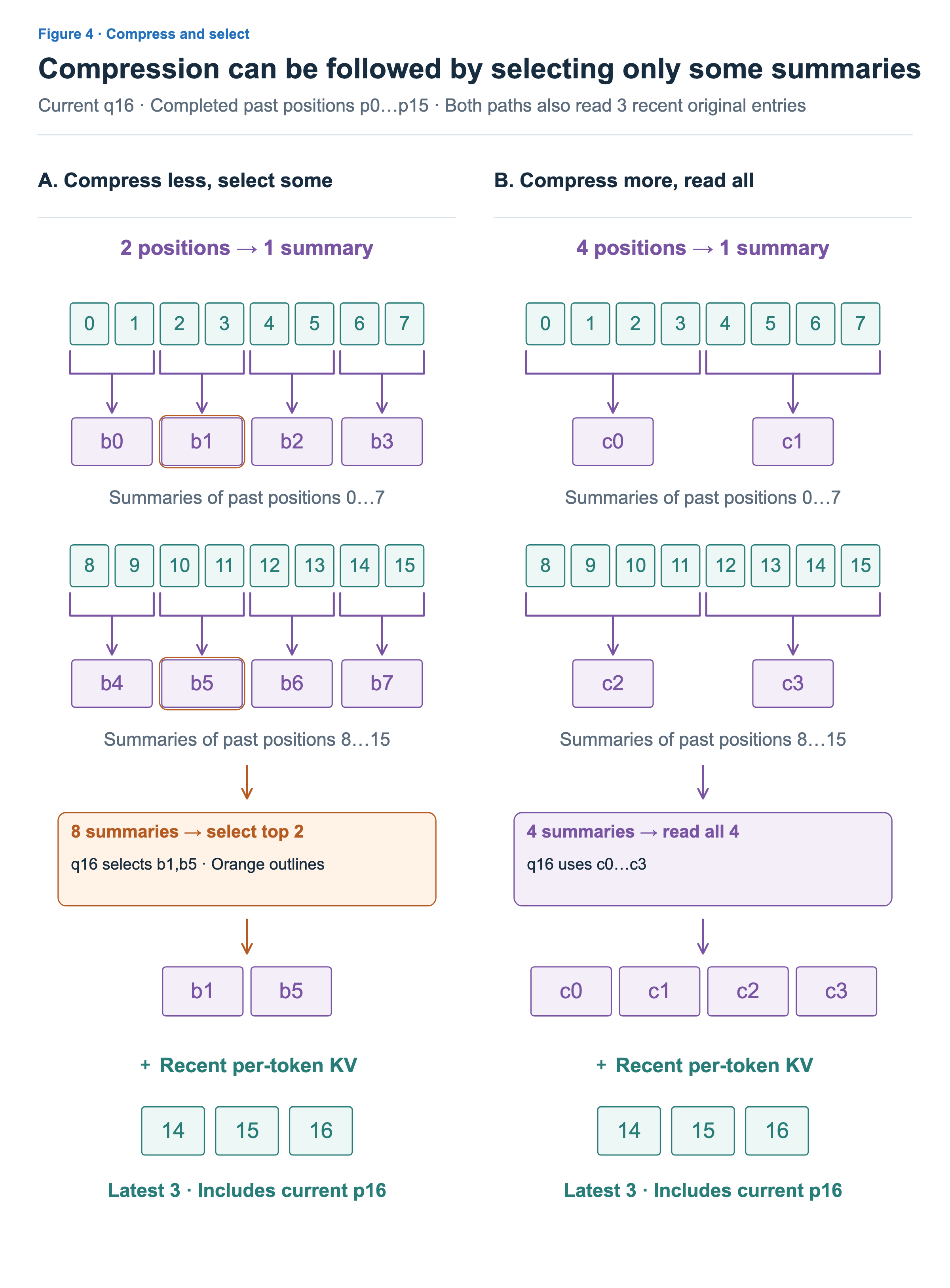
On the left, groups of two positions produce eight summaries. The indexer selects the Top-2 entries, $b_1$ and $b_5$. Summary $b_1$ represents positions 2 and 3, and $b_5$ represents positions 10 and 11. After selection, attention does not expand these back into the four original positions’ KV: it reads the two selected summaries themselves. Including the three recent per-token KV entries gives five read entries in this example.

On the right, groups of four positions produce four summaries, all of which are read. Adding the same three recent per-token KV entries gives seven read entries. Despite stronger compression, this example reads more entries than the left-hand path, because the left-hand path has a separate selection step. How many entries compression stores and how many of them attention reads must be distinguished.

The left-hand path does not retain only the two summaries being read now. It keeps eight summaries as candidates because the next query may select different ones. The right-hand path stores four summaries and reads them all. This educational example distinguishes storage from reading; it is not a performance comparison establishing that reading five entries must be faster than reading seven. The left-hand path also pays for indexer scoring and selection.

DeepSeek-V4’s official attention implementation combines compressed-entry indices with positions in the recent window. The groups of two and four in the figure do not reproduce the actual model’s compression ratios. The relationship to learn here is the distinction between selecting some compressed entries and reading all of a smaller set of summaries.

Larger groups yield fewer summaries, but each vector must hold information from more positions. An indexer cannot recover details that have already become difficult to distinguish during compression. The compression level, number of selected entries, and recent per-token KV window size therefore need to be chosen together. This trades the benefit of storing and reading fewer entries against how much useful information is retained.