Linear Attention: Accumulating KV in a Fixed-Size State

The previous article summarized KV from several positions before reading it. Even with summaries, the number of past entries grows with context length. Here we examine Linear Attention, which accumulates information in a fixed-size state instead of keeping a list of KV pairs for individual tokens.

The key is which computation comes first. Instead of first computing scores between a Query and individual Keys, we collect the relationships between Keys and Values and read them with the current Query. We cannot simply reorder ordinary softmax attention, however. We will first explain how the scoring rule changes, then follow writes and reads in a small matrix and the normalization that produces the final output.

From a KV list to a fixed-size state

Ordinary global attention appends the new position’s Key and Value to its cache when processing a token. It retains past KV so that the next Query can distinguish individual positions. Storage therefore grows with the number of tokens.

The right side of Figure 1 uses a different approach. Each new token updates a matrix of constant size, which we call state S. The figure shows one head in one layer. The matrices running down the figure show how the same state changes over time; they are not all retained.

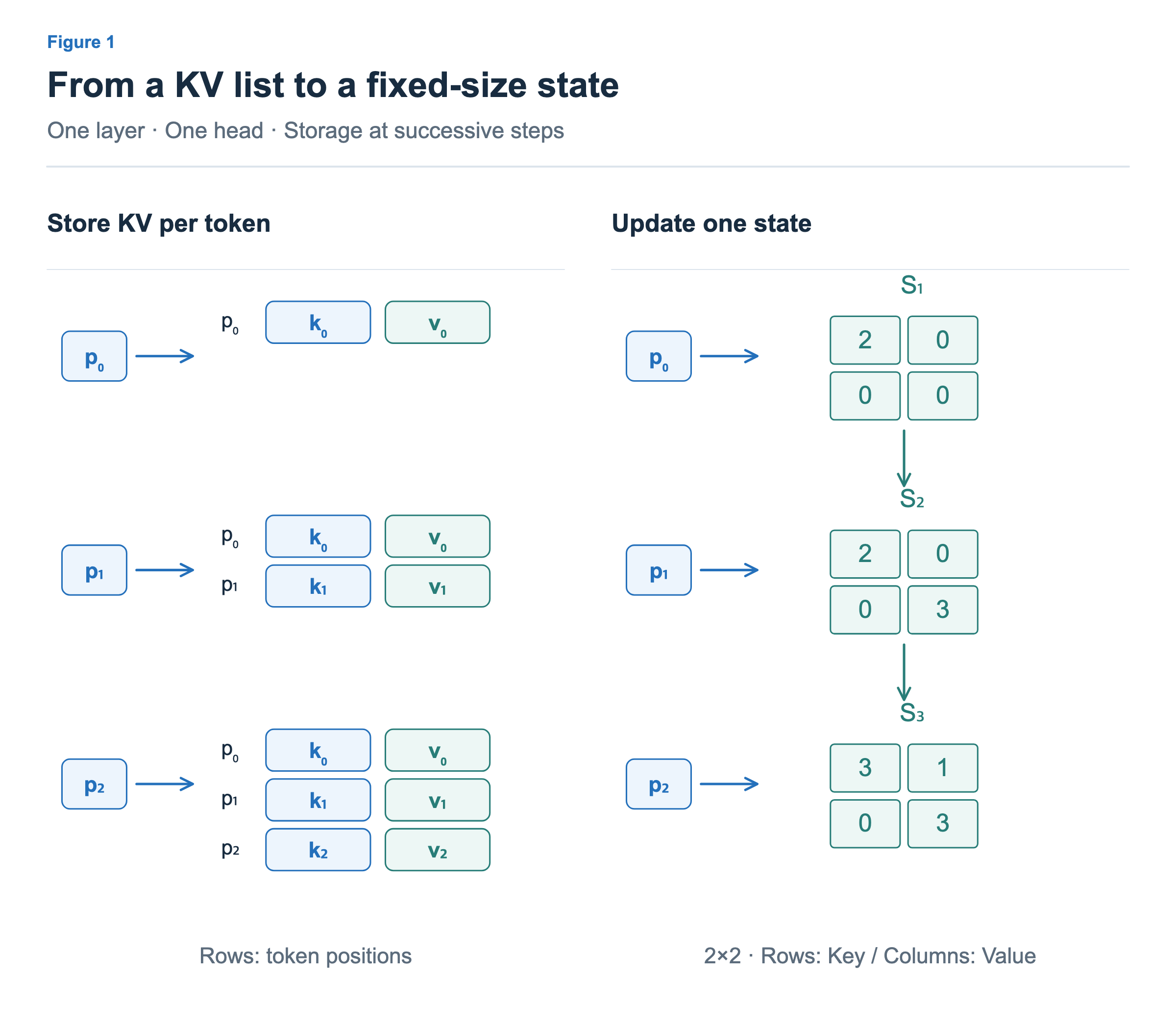
Rows in the KV list on the left are token positions. Rows and columns in the state on the right instead correspond to vector components. A row of the state does not represent one token. Contributions from several tokens are added to the same cells, so the matrix does not grow with the token count.

In this article, Keys and Values each have two components, giving a 2×2 state. We also maintain a small vector containing the sum of Keys for final normalization. We will first understand the matrix state and introduce this vector in the last figure. Constant storage here refers to the inference state that carries past context, not to all training intermediates or total model memory.

Why replace softmax?

In attention, a Value carries content, while Queries and Keys determine which content contributes and by how much. Ordinary softmax attention computes Query–Key dot products, scales them according to dimension, and applies softmax before combining Values.

For matrix multiplication alone, associativity gives (QKᵀ)V = Q(KᵀV). Actual attention, however, has softmax between the two products. The result of QKᵀ must enter softmax, so associativity alone cannot move KV computation first.

Could we just remove softmax? That would allow the products to be reordered. The issue is the scores’ properties. Softmax exponentiates dot-product scores to make them positive, then divides by their sum to obtain weights that sum to 1. Raw dot products can yield scores such as 1 and −1. One Value would then be added and another subtracted, and normalizing by the score sum would divide by zero.

Figure 2 separates these roles. Transform Queries and Keys independently into positive components, and use the dot product of the transformed vectors as the score. Normalization by the sum of scores is computed separately.

The transformation in the figure is a feature map, denoted by φ. The transformed Query is q̃ = φ(q), and the transformed Key is k̃ = φ(k). We do not combine the two vectors and transform them together: each is transformed independently. This is a separate step after the learned projections that produce Q and K from the input.

Section 3.2 of the original Linear Attention paper uses φ(x) = ELU(x) + 1, which makes each component positive. The dot product of the transformed Query and Key is then positive and can serve as the score in a weighted average.

The feature map itself does not enable associativity. Even φ(x) = x, with no transformation, allows the matrix products to be reordered. Reordering requires scores to be dot products of independently constructed vectors; a positive transformation is a choice about the scores’ properties. This article explains the variant that normalizes positive scores. Not all linear-attention variants use the same feature map or normalization.

This is also not merely an optimization that computes the same result as softmax more quickly. Changing the scoring function changes how much each Value contributes. The two outputs are generally different.

What computing KV first reduces

After changing the scores, the computation before normalization can take either of the two orders at the bottom of Figure 2. Q̃ and K̃ stack transformed Queries and Keys as rows in token order, and V stacks Values as rows.

$$\left(\mathrm{Q̃}{\mathrm{K̃}}^T\right)V=\mathrm{Q̃}\left({\mathrm{K̃}}^{T}V\right)$$

The left side computes scores between tokens first. For T tokens, Q̃K̃ᵀ is a T×T matrix. Each row is a Query position and each column a Key position, so doubling the token count quadruples the number of pairs.

The right side computes K̃ᵀV first. If a transformed Key has dₖ components and a Value has dᵥ components, the result is dₖ×dᵥ. This is the state S introduced earlier. The token-position axis is summed over in the multiplication, leaving relationships between Key components and Value components. Each Query then multiplies this state.

With fixed dimensions, the two products on the left require O(T²dₖ + T²dᵥ) operations, while the right side requires O(Tdₖdᵥ). On the right, every token adds a contribution to and reads a matrix of constant size, so total computation grows linearly with the number of tokens. This is what “Linear” refers to; it does not mean the feature map must be a linear function.

The comparison at the bottom of Figure 2 reads all positions to isolate the order of computation. Its small example uses transformed Query and Key rows [1, 0], [0, 1], and [1, 0], with Value rows [2, 0], [0, 3], and [1, 1]. Using this complete state at every position in a generation model would expose future information. Generation therefore reads a state accumulated only through the current position. We will now follow this process one token at a time.

Store Values according to Key components

In the remaining figures and equations, q and k denote vectors after the feature map to keep notation simple. The example’s zeros and ones are educational values chosen for easy arithmetic, not literal outputs of ELU+1. The examples use nonnegative scores and a positive denominator.

We process the following three tokens in order. Vectors are written horizontally in the table, but k and v in the equations are column vectors; the transpose symbol ᵀ changes their orientation.

Token position	Transformed Key	Value
p₀	[1, 0]	[2, 0]
p₁	[0, 1]	[0, 3]
p₂	[1, 0]	[1, 1]

First consider how one token contributes to the output. Take the dot product of the current Query and that token’s Key to obtain a score, then multiply the entire Value by it. This is the familiar “score × Value” calculation. Could we compute the Key–Value part before the Query arrives? Associativity makes that possible. The part grouped first is the outer product kvᵀ of the Key and Value. The outer product appears when we group KV first to compute the same weighted sum.

We are not taking a Key–Value dot product to obtain a single similarity score. A 2×1 Key column vector multiplied by a 1×2 transposed Value gives a 2×2 matrix. This product also works when Keys and Values have different numbers of components. A dot product multiplies corresponding components and sums them into a score; an outer product retains the products of every component pair as a matrix. Figure 3 shows the outer product for p₂.

The first Key component is 1, so the first row receives one times the entire Value: [1, 1]. The second Key component is 0, so the second row receives zero times the entire Value: [0, 0]. Each row contains the entire Value scaled by the corresponding Key component. The rows of this single outer product do not hold different content; they hold the same Value at different scales.

This is what “rows are Key components, columns are Value components” means. Each row corresponds to a Key component that determines the scale at which the Value is written, and its columns hold the Value’s components. A row number is neither a head index nor a token position.

If the Key were [0.3, 0.7] and the Value [1, 1], the first row would be [0.3, 0.3] and the second [0.7, 0.7]. Rather than selecting only one row, a general Key writes differently scaled copies of the same Value to several rows.

Add contributions to the same state

Initially, every state entry is zero. Each new token adds its outer product to the old state. Following the figures, S₀ is the empty state and S₁ is the state after processing one token. The state after processing position pₜ is therefore Sₜ₊₁.

In Figure 4, orange matrices are contributions from the current token, and green matrices are the accumulated states.

Token p₀ adds [2, 0] to the first row. Token p₁ adds [0, 3] to the second. Finally, p₂ adds [1, 1] to the first row, so S₃ has first row [3, 1] and second row [0, 3].

This accumulation equals stacking the tokens into matrices and computing KᵀV. Terms that matrix multiplication sums along the token axis are simply added one at a time as tokens arrive. Retaining only the state through the current position performs the same computation without reading future tokens.

The state stays 2×2 as tokens are added. Their contributions share its cells: the first row [3, 1] alone cannot reconstruct the original [2, 0] and [1, 1] separately. A fixed-size state is not a lossless copy of the KV list. But recovering individual KV pairs and computing the required weighted sum from them are different questions. The weighted sum under this scoring rule is exactly the same as when retaining individual KV pairs. The next figure compares the two computations.

Read the state with a Query

Reading means using the Query components as weights for summing the state’s rows. If the current q₂ is [1, 0], we add one times the first row and zero times the second.

The left side of Figure 5 gives 1 × [3, 1] + 0 × [0, 3] = [3, 1]. A Query of [0, 1] reads the second row, [0, 3], while [1, 1] sums both rows to [3, 4]. These are weighted sums before normalization.

When writing, we scaled the Value in each row by a Key component. When reading, we multiply that row by the corresponding Query component and sum. The Key sets the write scale, and the Query sets the read scale. For one token’s contribution, the two scales multiply in each row; summing those products gives the Query–Key dot product.

Reading the state therefore weights each token’s Value by its Query–Key score. Expand the contributions by token, as on the right side of the figure. The dot products of q₂ = [1, 0] with the three Keys are 1, 0, and 1. Multiplying each Value by its score gives:

1 × [2, 0] + 0 × [0, 3] + 1 × [1, 1] = [3, 1]

This matches the left side. The relationship holds for an accumulation of outer products, not just for one pair. Matrix multiplication distributes over addition, so adding the outer products before multiplying by the Query gives the same result as multiplying each first and then adding. Expanding the accumulated state gives:

$${q_t}^T{S}_{\mathrm{t+1}}=\sum _{i=0}^t\left({q_t}^T{k}_i\right){v_i}^T$$

In other words, writing Values according to Key components and reading the state according to Query components weights each Value by the corresponding Query–Key dot product. We can compute this weighted sum without comparing the current Query with every past Key individually again.

We can thus compute the required weighted sum without reconstructing the original KV pairs. This equality concerns the dot-product scores chosen in this article; it does not assert equality with softmax attention.

Divide by the sum of scores

Why divide the [3, 1] in Figure 5 rather than use it directly as the final output? The attention variant explained here returns a weighted average of Values. Softmax weights already sum to 1, but the dot-product scores 1, 0, and 1 sum to 2. Dividing the weighted sum by 2 gives an average with weights 0.5, 0, and 0.5.

Consider a Value [2, 0] with score 1. Adding it once gives [2, 0], while adding two copies gives [4, 0]. Dividing by the score sum gives [2, 0] in both cases. This reduces growth in output magnitude caused merely by reading more copies of the same content. The division does not reverse information loss in the state.

Without storing individual Keys, how do we obtain the score sum? Accumulate a vector z containing the sum of Keys alongside the matrix. Figure 6 shows the numerator and denominator together.

The sum of the three Keys is z₃ = [1, 0] + [0, 1] + [1, 0] = [2, 1]. Its dot product with q₂ = [1, 0] is 1 × 2 + 0 × 1 = 2, exactly the sum of the Query’s dot products with each Key.

The final output is [3, 1] ÷ 2 = [1.5, 0.5]. The denominator 2 is the sum of scores for the current Query, not the token count 3. A different Query can produce a different denominator from the same z.

Summarize state updates and reads with equations

First, confirm why the outer product appears. One token contributes the Query–Key dot product times its Value. Reordering the products gives:

$$\left(q^{T}k\right)v^T=q^T\left(k{v}^T\right)$$

The left side computes the score first; the right side forms the outer product first. That matrix records the Value at the scale of each Key component, and multiplying by qᵀ reads it at the scale of each Query component. Since this holds for every token, we can accumulate outer products in a state and read them together.

The process is “add the current Key–Value relationship to the state, then read the updated state with the Query.” We use Sₜ for the state before processing position pₜ and Sₜ₊₁ for the state afterward. The state subscript counts processed tokens, while the subscript of output yₜ is the current input position. We will use the same convention for SSM and Mamba. Below, q and k are column vectors after the feature map.

$$S_{t+1}=S_t+k_t{v_t}^T$$

On the right, Sₜ contains contributions from earlier tokens, and kₜvₜᵀ is the current token’s outer product. We leave the old state intact and add the new contribution. We accumulate this way because, as Figure 5 showed, reading with a Query yields the sum of Values weighted by their Query–Key dot products. The state is constructed to compute that weighted sum, rather than defined arbitrarily and then read.

To make the final output a weighted average, we update the Key sum z in the same order. Both S₀ and z₀ start at zero.

$$z_{t+1}=z_t+k_t$$ $${y_t}^T=\frac{{q_t}^T{S}_{t+1}}{{q_t}^T{z}_{t+1}}$$

The numerator is the weighted sum read from the state by the current Query, and the denominator is the sum of scores for that Query. In Figure 6 they are [3, 1] and 2, giving y₂ = [1.5, 0.5]. We define y as a column vector with the same dimension as a Value, so the left side is yₜᵀ to match the row vector on the right. The transpose indicates vector orientation; it is not another normalization operation.

With a positive denominator, this equation exactly computes the weighted average of Values under this article’s scores. It does not reproduce ordinary softmax attention. Per head, storage consists of dₖ×dᵥ matrix components and dₖ vector components. Section 3.3 of the original paper also expresses causal attention through these two accumulated quantities.

Benefits and limits of a fixed-size state

With fixed dimensions, updating and reading the state for one token does not grow in cost with the number of past tokens. Total attention computation for T tokens grows linearly with T. The matrix dimensions still contribute to cost, and actual speed depends on dimensions, implementation, and parallelization.

Not constructing a T×T score matrix does not mean ordinary attention must store that entire matrix in memory. Some implementations process scores in tiles. This article changes the scoring function and computational structure, not just how an intermediate matrix is stored.

A fixed-size state still computes the weighted sum for this scoring rule exactly. The remaining question is whether continually adding each new contribution is the right write rule. Different Values arriving under the same Key accumulate old and new content together. That suits summing or averaging them, but moving the readout for that Key toward a new Value requires a different update rule.

The next article’s delta rule checks what the old state returns and applies the difference from the new Value. It does not repair a weighted sum corrupted by accumulation. It changes the write rule from adding new contributions to making corrections based on the existing readout.