The Delta Rule: Revising State Associations Toward a New Value

The previous article added outer products of Keys and Values to a fixed-size state and read that state with a Query. Even after accumulation, the Value weighted sum using Query–Key dot-product scores is exactly the same as when computing with individual KV pairs.

This article focuses on how to change the state when a new KV pair arrives, rather than on the result of that computation. Instead of continually adding new content, the delta rule compares it with what the state currently returns and applies the required change.

The delta rule does not repair a weighted sum that went wrong during accumulation. It chooses a write rule: keep adding new contributions, or revise the existing readout toward the new Value. Before learning how to calculate the difference, we need to understand its purpose. Why does the new Value serve as the target for the update, and why do we read the old state with a Key rather than a Query? We will first distinguish writing KV associations from computing an output with a Query, then examine the write rule chosen by the delta rule.

Write with KV, read with a Query

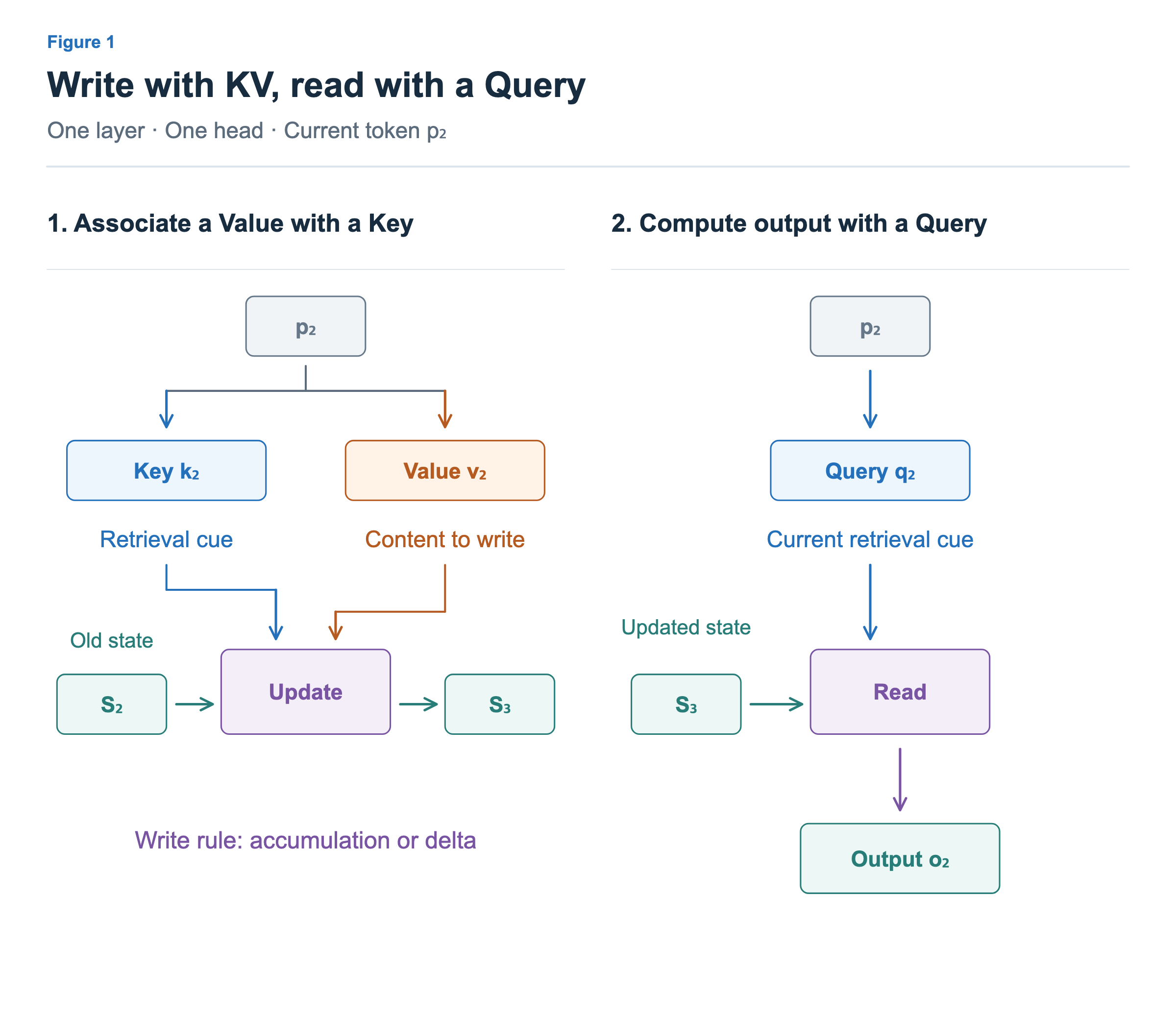
Consider the Key and Value produced from the current token as a pair. The Value is the content to write, and the Key determines the scale at which it contributes to each state row. A Query applies a read scale to each row. Summing the products of write scales and read scales gives the Query–Key dot product. Adding their outer product in the previous article served the same purpose: when a future Query matches this Key, this Value should contribute to the output.

The Query that reads the state has a different role. It retrieves information for the current output. Even when a token supplies the Key, Value, and Query, they use different projections, so its Key and Query need not be the same vector. Deciding what to write and what to read now are different roles.

Figure 1 separates these two processes. The Key and Value of the current token $p_2$ update the old state $S_2$ into $S_3$. The current Query $q_2$ then reads $S_3$. In this article, the state subscript counts the tokens processed: $S_2$ includes the two preceding tokens, and $S_3$ includes the current token $p_2$ as well.

Writing the current token before reading the state allows the output to incorporate information through the current position. This is the same visibility range as ordinary causal attention, which includes the current position. Each state block in the figure represents an entire matrix, not a storage slot reserved for a particular token.

Add new content or revise an association?

When writing a new Value for the same Key, we can choose between two objectives. One is to add a new contribution to the old state. The other is to change the state so that reading it with this Key returns a value closer to the new Value. The delta rule follows the second objective.

Why is the new Value the target? The current KV pair represents the association we want to write: this Value should be readable through this Key. The delta rule writes that association by applying the difference between the current readout and the new content. The new Value is not an externally supplied correct answer, nor is it necessarily more correct than the old content. It is the target of the state update because it is the content we are currently trying to write.

Suppose reading the old state with this Key returns [2, 0], and the new Value is [1, 1]. Additive accumulation adds the new contribution. The delta rule instead takes the existing readout [2, 0] into account and moves it toward [1, 1]. Computing and applying this difference between the target and the current value is the basic idea of the delta rule. Section 2.2 of the DeltaNet paper likewise updates the state using the difference between the new Value and the old readout for the current Key.

If the readout already equals the new Value, the difference is zero. The delta rule has no further correction to make to that association. Additive accumulation, in contrast, adds another contribution even when the same content arrives again. Neither is universally correct; they use different rules for incorporating new information into the state. What changes here is the state holding the context, not the model’s projection weights being retrained during inference.

Why read with a Key, and why read with a Query?

The previous article read the state with a Query. Why use a Key here? We need to inspect the association we are about to change. Before updating, the question is “What does the current state return when read with this Key?” We need that value to calculate how far it is from the Value we want to write.

This does not mean searching for an identical Key stored in the past and retrieving one entry. The state contains combined contributions from many tokens. Like a Query, the current Key takes a weighted sum of the state’s rows to produce a vector. The readout can therefore be nonzero even if this exact Key has never appeared before. An “existing associated value” means the value that the current state returns for this Key.

Reading with a Key and reading with a Query have the same computational form: multiply a vector by the state. What differs is the vector used, when the read occurs, and what the result is for.

Aspect	Read with the current Key	Read with the current Query
Which state is read?	State before the update	Updated state
What is retrieved?	What is already readable through this Key	Information for the current output
How is the readout used?	Compare with the new Value to compute a correction	Compute the output

The order is read the old value with the Key → compare with the new Value and update the state → compute the output with the Query. We do not first add the new Value and then repair a mistake. We inspect the current value before writing to determine the change to apply.

Also, the actual output does not have to equal the new Value. Suppose the updated state’s first row is [1, 1] and its second row is [0, 3]. The writing Key [1, 0] reads the first row, [1, 1]. But a current Query of [0, 1] produces the second row, [0, 3]. The vector used to check the association and the vector used to retrieve information for the output are different. This article considers direct state readouts; it does not carry over the score-sum normalization from the end of the previous article.

With that distinction in mind, consider Figure 2. Both sides start from the same old state, with Key [1, 0] and new Value [1, 1]. Reading the old state with this Key returns [2, 0]. The left side adds the new contribution and then reads [3, 1]. The right side revises the association to read [1, 1]. The right-hand result exactly matches the new Value because this example uses a unit-length Key and correction strength β=1.

The label “Check the write with the same Key” at the bottom is a check used to illustrate the difference between the two write rules. An actual execution does not have to read with the same Key again after the update as a verification step. The Key read needed for the update happens before it; the actual output after the update is read with the Query.

Write the difference between the readout and the new Value

We can now work out how to obtain the right-hand result in Figure 2. The first row of the old state $S_2$ is [2, 0], and its second row is [0, 3]. Reading with the current Key $k_2$ = [1, 0] weights the first row by 1 and the second by 0, returning [2, 0].

The new Value is [1, 1]. Adding it directly would give a readout of [3, 1], but our objective is to change the readout for this Key to [1, 1]. The required change is therefore new Value − current readout = [1, 1] − [2, 0] = [−1, 1]. The first component must decrease by 1, and the second must increase by 1.

Figure 3 applies this difference to the state and checks the result with the same Key. For now, we apply the full correction; the next section adjusts the fraction applied.

The difference is a two-component vector, while the state is a 2×2 matrix. How much should we add to each row? Just as we took the outer product of the Key and Value in the previous article, we now take the outer product of the same Key and the difference vector. With Key [1, 0], we add one times the difference, [−1, 1], to the first row and zero times it, [0, 0], to the second.

State row	Old value	Correction to add	After update
First row	[2, 0]	[−1, 1]	[1, 1]
Second row	[0, 3]	[0, 0]	[0, 3]

Reading the updated $S_3$ with the same Key [1, 0] returns the first row, [1, 1]. The final multiplication by the Key does not force an output to match the new Value. We have changed the state itself so that reading with that Key returns the new Value.

Only the first row changes here because the Key is [1, 0]. A general Key has several nonzero components, so the difference is added to multiple rows with different weights. This is not equivalent to replacing a slot reserved for a specific token.

In notation, let rᵀ be the row vector read with the current Key, and eᵀ the difference from the new Value. This article uses state rows for Key components and columns for Value components, so reading is kᵀS and writing is keᵀ.

$$r^T={k_t}^T{S}_t$$ $$e^T={v_t}^T-r^T$$

Here, $S_t$ is the state before writing the current token, and $k_t$ and $v_t$ are its Key and Value. The vector r is computed by reading the current state with this Key, not by looking up a separately stored past Value.

Adjust the correction strength with β

We can apply the full change toward the new Value at once, or retain some of the old readout and incorporate only part of the new content. To do this, multiply the correction by the update fraction β. This section compares values of β between 0 and 1.

$$S_{\mathrm{t+1}}=S_t+\beta k_t{e}^T$$

We do not multiply the entire new Value by β and add it. We multiply the difference between the new Value and the current readout by β. All three cases in Figure 4 start from the same $S_2$; they are not three successive updates from top to bottom.

With β=0, the correction is [0, 0], leaving the first row [2, 0] unchanged. With β=0.5, we add half of the difference [−1, 1], or [−0.5, 0.5], to obtain [1.5, 0.5]. With β=1, we apply the full difference to obtain [1, 1]. Reading with the same Key returns these respective values.

In this example, the readout moves between the old value and the new Value. This interpretation assumes that the Key has unit length. Reading the correction with the same Key multiplies the difference vector by β and kᵀk. A unit-length Key has kᵀk=1, so β is the fraction of the difference applied. This is why β=1 exactly matches the new Value. Arbitrarily scaled Keys do not always produce the same result.

In an actual model, β can be computed from the input rather than chosen manually each time. The values 0, 0.5, and 1 in the figure illustrate its role. Section 2.2 of the DeltaNet paper uses an input-dependent update strength and also discusses Key normalization.

Reducing β makes this correction smaller and changes the old state less. It does not guarantee that a fixed proportion of all past information is preserved. Contributions from multiple tokens share the state’s rows, and other Queries can read the parts that changed.

How a state update affects other reads

Even when the delta rule corrects the readout for the current Key, the correction does not apply independently to that Key alone. Readouts for other Queries can change too. The state has no separate storage slot for every Key: contributions from multiple tokens overlap in the same matrix. If another Query reads a part changed for the current Key, its result reflects that change.

The earlier correction for Key [1, 0] changed the first row from [2, 0] to [1, 1] and left the second row [0, 3] unchanged. A Query reading only the second row is therefore unaffected, while a Query that also reads the first row produces a different result. Figure 5 shows the before-and-after readouts in these two cases.

The left Query [0, 1] weights the first row by 0 and the second by 1. The changed first row contributes nothing, so the readout remains [0, 3].

The right Query [1, 1] reads both rows. Before the correction, it returns [2, 0] + [0, 3] = [2, 3]; afterward, it returns [1, 1] + [0, 3] = [1, 4]. Although this Query differs from the writing Key, it reads the changed row and therefore returns a different value. The Query [1, 1] illustrates a weighted sum of rows; it is not a unit-length vector.

The difference between the cases is how much the Query reads the modified part. Revising an association toward a new Value and preserving other readouts are separate matters. A change in another readout is not always wrong, but we cannot guarantee that revising one association leaves every other read unchanged.

The same relationship follows from the computation. If the state correction is βkeᵀ, the change in the readout for Query q is β(qᵀk)eᵀ. If the Query’s dot product with the current Key is zero, this correction has no effect on its readout. Otherwise, the difference contributes in proportion to that dot product. The dot products are 0 on the left and 1 on the right.

The delta rule keeps the fixed-size state structure while revising writes relative to the existing readout instead of simply adding new content. The next article will add a step that controls how much of the old state to retain before applying this correction.