GDN and KDA: Retaining State and Applying Delta Corrections

The previous article introduced the delta rule: read the state with the current Key and apply a correction that moves that readout toward the new Value. This article adds control over how much of the old state to retain. We will first consider why writing new content also calls for a way to reduce the influence of information already accumulated.

Gated DeltaNet (GDN) applies a retention rate to the old state before performing a delta correction. Kimi Delta Attention (KDA) applies different retention rates to different state components. We will compare them using small matrices, then connect these controls to how the model computes retention and correction strength from the current input.

Why control how much of the old state remains?

The delta rule aims to make the readout for the current Key closer to the new Value. In the previous example, Key [1, 0] read the first row of the state, and the correction added the difference only to that row. The second row remained unchanged.

When the context changes, however, we may want to reduce the influence of other information in the old state as well as update the association for the current Key. Reducing the delta rule’s β cannot accomplish this by itself. β determines how much of the current correction to apply. Setting β=0 leaves the state unchanged; it does not reduce the old content.

GDN therefore multiplies the old state by a retention rate α. An α close to 1 retains much of the old state; an α close to 0 greatly reduces it. This combines control over retaining the old state with control over correcting it toward the new Value. Section 3.1 of the Gated DeltaNet paper combines state decay and delta correction to serve these two roles.

Figure 1 starts both cases from the same state and writes the same Key [1, 0] and new Value [1, 1]. Both use β=1 for correction. Only the right side first retains half of the old state.

The left side applies only the delta rule, changing the first row from [2, 0] to [1, 1] while leaving the second row [0, 3] unchanged. The right side first multiplies the entire state by 0.5, then corrects it. Its first row also becomes [1, 1], but its second row shrinks to [0, 1.5]. Retention can reduce parts of the state that the correction for this Key does not touch.

This example does not mean that the second row contains unnecessary information. Reducing useful information can harm later reads. The point is that we now have a separate means of reducing the influence of old information. Also, a general Key reads and changes multiple rows. Only the first row changes here because this example uses Key [1, 0].

Apply the delta correction to the retained state

GDN proceeds in this order: apply retention to the old state → read the retained state with the Key → compute the difference from the new Value → apply β of the correction. The crucial point is that the read used to compute the difference comes from the state after retention.

As in the previous article, Figure 2 starts with $S_2$, which incorporates two tokens, and processes the current token $p_2$ to produce $S_3$. Rows are Key components and columns are Value components. We use α=0.5 and β=1, and denote the intermediate state after retention by $\overline{S}$.

Multiplying the old state’s first row [2, 0] and second row [0, 3] by α=0.5 gives [1, 0] and [0, 1.5]. Reading this state with the current Key [1, 0] returns the first row, [1, 0].

The new Value is [1, 1], so the required difference is [1, 1] − [1, 0] = [0, 1]. Taking the outer product of the same Key and this difference gives a correction that adds [0, 1] to the first row and [0, 0] to the second. With β=1, we apply all of it, yielding a final first row of [1, 1] and second row of [0, 1.5].

If we instead read [2, 0] before applying retention, the difference would be [−1, 1]. Adding that to the already reduced first row [1, 0] would give [0, 1], which differs from the intended [1, 1]. Because the state being corrected has changed, we must compare the readout from that state with the new Value.

Following the previous article’s notation, let $S_t$ denote the state before writing the current token. We can express the steps as follows. Here, rᵀ is the readout from the retained state, and eᵀ is the difference from the new Value.

$$\overline{S}={\alpha }_t{S}_t,r^T={k_t}^T\overline{S}$$ $$e^T={v_t}^T-r^T$$ $$S_{t+1}=\overline{S}+{\beta }_t{k}_t{e}^T$$

α and β act on different parts of the update. α multiplies the old state before correction, whereas β multiplies the correction that writes the difference between the new Value and the readout. For example, with α=0.5 and β=0, no delta correction occurs, but the old state is still halved. With α=1, the old state is retained in full and only the delta rule is applied. The values 0 and 1 are boundary cases used to distinguish these roles.

In this example, reading with the same Key after a β=1 correction returns exactly the new Value because Key [1, 0] has unit length. The actual output still comes from reading the updated state with the current Query. That output does not have to equal the new Value.

KDA: retention rates for individual components

GDN multiplies an entire head’s state by the same α. For example, α=0.5 halves every row. But we may want to retain more of some components and reduce others more strongly. A single retention rate cannot express this difference.

KDA computes a retention rate for each Key component. With the state convention used here, where rows are Key components, this means multiplying each row by a different retention rate. Section 3 of the Kimi Linear paper extends GDN’s scalar decay to component-wise decay.

The left side of Figure 3 is GDN. Both rows are multiplied by 0.5, giving [1, 0] and [0, 1.5]. The right side is KDA. It multiplies the first row by 0.9 to retain [1.8, 0], and the second row by 0.2 to retain [0, 0.6]. It can retain more of the first component while reducing the second more strongly.

These are states after retention only, before correction. KDA then reads this state with the current Key and applies β of the correction toward the new Value. The delta rule remains; what becomes more detailed is how the old state is retained before correction.

Do not interpret a row as one past token or one independent memory. Each row combines contributions from multiple tokens. Component-wise retention therefore does not select a particular token to erase, and it can affect multiple Queries that read the reduced components. The previous article’s explanation that a β-scaled correction can affect other reads still applies.

Compute retention and correction strength from the input

So far, we have chosen values such as α=0.5 and β=1 for the examples. In an actual model, a person does not choose these values at each step. The model projects the current token’s vector with learned weights and transforms the results to compute α and β for this token.

Think of this in the same way as producing Q, K, and V. The weights that produce a Query are learned, while the Query itself is computed from the current input. Likewise, the weights that produce α and β are learned parameters, while α and β are values computed using those weights and the current input.

The left side of Figure 4 shows how these controls are produced; the right side shows where they are used. The $p_2$ block on the left represents neither the position number 2 nor a token ID, but the entire vector representing the token at that position as it enters the current layer.

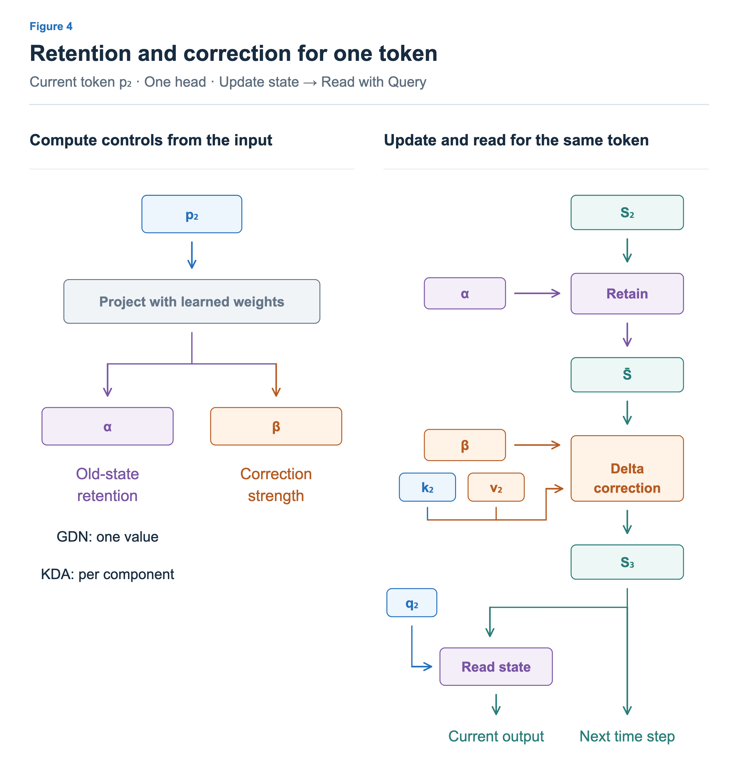
The figure abbreviates this as “Project with learned weights,” but the projected values also undergo transformations that control their range before being used as retention or correction rates. For example, in Section 4 of the Kimi Linear paper, β is computed by applying sigmoid to a weighted projection of the current input. α is produced for each Key component through two projection stages and a decay function.

Quantity	During training	During inference
Weights that produce α and β	Learned together with the model’s other weights	Use the learned values
α and β for the current token	Computed from the current input	Computed from the current input

Even after training fixes the weights, different inputs can produce different α and β values. GDN’s α is one value computed per token and per head; KDA’s α is a vector with a separate value for each Key component within a head. In both methods, β is a scalar controlling the strength of the current correction within a head.

The flow on the right first uses α to retain the old state, then performs the delta correction with the current Key, Value, and β. The updated $S_3$ becomes the state carried forward to process the next token. The current Query also reads this state to produce a value for the current output. Retention, correction, and reading are not assigned to different tokens: they all occur while processing the current token.

This lets the model adjust how much old information to retain and how strongly to incorporate new content based on the input, without increasing the size of the state. It still records information from multiple tokens in the same state, however. Finer-grained retention does not turn that state into a store of individual past KV pairs from which a chosen token can be read directly.