SSMs: Carrying Context Through State and New Inputs

The Linear Attention family covered through the previous article writes past information into a fixed-size state and reads that state with the current Query. An SSM (State Space Model) also carries past information forward in a state. How does it differ from what we have already learned?

We will connect the two approaches through the operations that retain state, write new information, and read an output. We will first examine an SSM with fixed coefficients, then calculate a small state vector to see how past inputs continue to contribute. Mamba, the subject of the next article, makes these coefficients depend on the current input.

From Linear Attention to SSMs

Basic Linear Attention adds the outer product of a Key and a Value to the state. Reading with a Query combines past Values according to the similarity between the Query and each Key. In that explanation, the state is a memory holding multiple Key–Value associations together.

SSMs reach a similar state-based structure from a different starting point: represent the influence of the past in the current state, and model how that state changes when it receives a new input.

Imagine supplying heat to an object that is hotter than its surroundings. If the state is its temperature difference from the surroundings, the influence of existing heat diminishes over time while the heater adds heat. We can describe the next state as “the result of changing the existing state + the influence of a new input.”

The linear SSM considered here chooses to express these two influences with matrix multiplication and addition. This does not mean that every system must follow this rule. In a language model, the state need not represent a physical quantity such as temperature. The weights are learned so that it holds past information useful for next-token prediction.

An SSM also adds a new contribution to the previous state, then reads an output from the updated state. The fixed-coefficient SSM we will examine specifies this process with three operations. $\overline{A}$ transforms the previous state, $\overline{B}$ turns the current input into a contribution to write, and C reads an output from the state. Figure 1 aligns the two approaches in the same order.

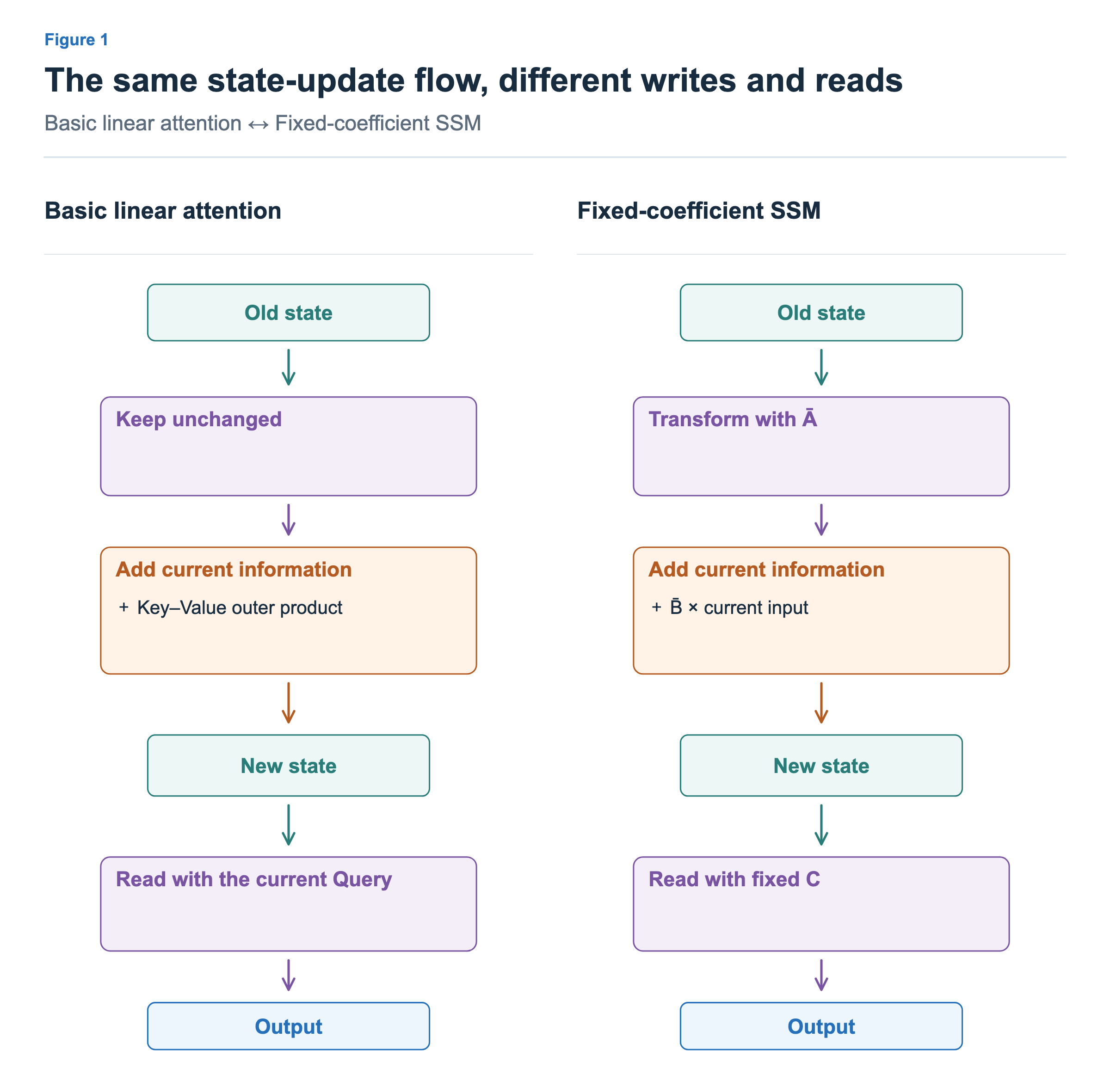
Basic Linear Attention leaves the previous state unchanged before adding a new Key–Value contribution. In the SSM, $\overline{A}$ acts on the previous state before new information is added. Depending on its values, $\overline{A}$ can reduce state components or mix them. Our small example will use different coefficients for the individual components.

Writing and reading also differ. Linear Attention writes with the Key and Value derived from the current input and reads with a Query. The fixed-coefficient SSM writes the input transformed by $\overline{B}$ and reads with C. $\overline{B}$ and C remain the same even when the input changes during inference. To focus on the update structure, the figure omits Linear Attention’s denominator normalization and the SSM term that adds the input directly to the output. Linear Attention paper, Mamba paper §2

We have already seen the previous state being reduced in GDN and KDA. State decay is therefore not a concept that first appears with SSMs. Focus instead on which update rule defines the state-based computation.

Figure 1 uses the same “state” block on both sides to compare their shared structure. Later, we draw the SSM state as a small vector because we are zooming in on one channel. The difference between a matrix in Linear Attention and a vector in this SSM example is not the essential distinction between the two approaches.

Combining the previous state with a new input

Consider processing one input channel in a layer. Let u be the input value in this channel and h the state holding the influence of past inputs. Here, u is a component of a feature vector representing a token, not a token ID or position number. We will give h two components: two memory components used to process one input component.

Suppose the previous state is [2, 1] and the current input u is 2. We retain 0.5 times the first state component and 0.8 times the second. We write 1 times the input into the first component and 0.5 times the input into the second. Finally, we read the output by summing the two state components.

First, apply $\overline{A}$. Multiplying the components of [2, 1] by 0.5 and 0.8 gives [1, 0.8]. This is the past contribution retained at this step. In this example, $\overline{A}$ is a 2×2 matrix with diagonal entries 0.5 and 0.8 and zeros elsewhere. The figure’s “× [0.5, 0.8]” is a compact way of showing this diagonal matrix acting on each component.

Next, apply $\overline{B}$. $\overline{B}$ is a column vector with components 1 and 0.5, so multiplying it by the scalar input 2 gives [2, 1]. One current input is written into several state components at different scales. Adding this to the retained [1, 0.8] produces the new state [3, 1.8].

Now read with C. With C=[1, 1], multiply each new state component by 1 and sum them: 3 + 1.8 = 4.8. If C were [1, 0], we would read only the first component, 3. The operation that constructs the state is separate from the operation that chooses what to read out.

Why one input persists at different rates

To see how long an input’s influence lasts, provide one nonzero input and set subsequent inputs to 0. With no new contribution being added, we can observe how the previous state changes.

Start from [0, 0] and provide input 2 at position p₀. Using $\overline{B}$ from the previous section gives the first state h₁=[2, 1]. Set the inputs at p₁ and p₂ to 0 and repeatedly apply the same $\overline{A}$. Each bar in Figure 3 shows one component of the same state vector changing over time, not one token.

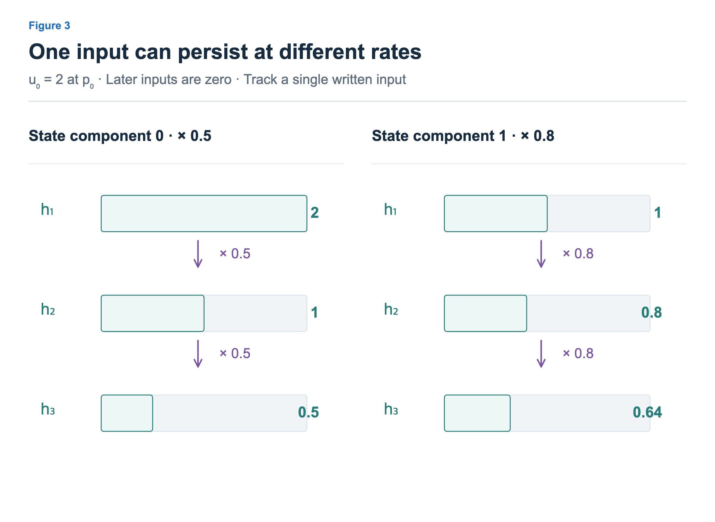
The first component is multiplied by 0.5 at each step: 2 → 1 → 0.5. The second is multiplied by 0.8: 1 → 0.8 → 0.64. Both contributions came from the same input 2, but its influence lasts longer in the second component. With C=[1, 1], the outputs are 3, 1.8, and 1.14.

Components with different rates of change let one state contain components that strongly reflect recent inputs and others that retain older influences. When new inputs keep arriving, each component accumulates contributions from multiple inputs. A component should therefore not be interpreted as a storage slot for one particular token.

The coefficients 0.5 and 0.8 were chosen to explain the principle. They are not actual Mamba coefficients or measured memory durations. Nor does every SSM simply decay like these two components. This is a minimal example for examining how a state transition changes the influence of past inputs.

What fixed coefficients mean

So far, $\overline{A}$, $\overline{B}$, and C have been fixed independently of the current input. If the input changes from 2 to −2, the written contribution and the new state change, but the coefficients themselves do not.

Figure 4 processes two inputs starting from the same previous state [2, 1]. Both cases retain [1, 0.8] through $\overline{A}$ and use the same $\overline{B}$ and C.

Input 2 adds [2, 1], producing [3, 1.8]. Input −2 adds [−2, −1], producing [−1, −0.2]. Reading with C=[1, 1] gives 4.8 and −1.2, respectively.

The input value affects the result, but the model does not use its content to compute new retention, write, and read coefficients. This is what fixed coefficients mean here. It does not mean the coefficients never change during training. It means the trained model applies the same coefficients at every position during inference.

Expressing the update and read as equations

Let us collect the illustrated process into equations. The memory denoted by S in Linear Attention is represented here by a single-channel state vector h. The state has a different name, but the temporal order stays the same. We use y for the output, as in the Linear Attention article; here it is a scalar output for one channel.

Write the state before processing the current input as $h_t$ and the state afterward as $h_{t+1}$. The state subscript counts the inputs processed so far.

$$h_{t+1}=\overline{A}{h}_t+\overline{B}{u}_t$$ $$y_t=C{h}_{t+1}$$

The bars over $\overline{A}$ and $\overline{B}$ indicate coefficients used in a discrete update that processes one token at a time. Although the figures arrange state components horizontally for readability, h and $\overline{B}$ in the equations are 2×1 column vectors, and C is a 1×2 row vector. After the new state is read to produce an output, it remains available to process the next input.

In the first equation, $\overline{A}$hₜ transforms the previous state into its retained contribution, while $\overline{B}$uₜ turns the current input into a contribution to write. They correspond to [1, 0.8] and [2, 1] in Figure 2. Adding them gives [3, 1.8], and reading with C in the second equation gives 4.8.

Here, uₜ is one channel of the input features supplied to the SSM. A neural network may create these features through projection and other operations, but the equation itself does not specify that preceding computation. $\overline{A}$hₜ transforms the state holding past information; it is not a projection of the input token. The two paths meet at the addition.

Expanding the recurrence reveals past inputs

Expanding a few steps shows why this update can carry context. Set the initial state h₀ to 0 and repeatedly use the same $\overline{A}$ and $\overline{B}$:

$$h_1=\overline{B}{u}_0$$ $$h_2=\overline{A}\overline{B}{u}_0+\overline{B}{u}_1$$ $$h_3={\overline{A}}^2\overline{B}{u}_0+\overline{A}\overline{B}{u}_1+\overline{B}{u}_2$$

The state h₃ contains contributions from all three inputs. The most recent input contributes $\overline{B}$u₂. The contribution from u₁ has passed through $\overline{A}$ once, and the contribution from u₀ has passed through it twice. Older inputs remain in a form that has undergone more state transitions.

Figure 3 follows only the first input’s contribution by setting later inputs to 0. A component with a diagonal coefficient of 0.5 halves at each step; one with 0.8 declines more slowly. Combining components with different rates of change lets the state represent past influences over different time ranges, and C combines those components into an output. This structure alone does not guarantee that important context will be preserved well. What is written and read depends on learning, state size, and the coefficient structure.

Linear Attention adds kₜvₜᵀ directly to the previous state. This SSM applies $\overline{A}$ to the previous state and adds $\overline{B}$uₜ. It also reads with fixed C rather than the current Query. $\overline{A}$, $\overline{B}$, and C have no time subscript because they are the same at every position during inference. In the next article, these coefficients will depend on the input.

We may want to incorporate a new input more strongly or retain more of the existing state depending on context. Mamba, covered next, enables this choice by computing coefficients from the current input. It preserves the structure of carrying, writing, and reading state while changing how that structure responds to the input.