Mamba: Choosing What to Remember Based on the Input

The SSM article transformed the previous state, added the current input’s contribution, and read an output from the new state. Even with the same coefficients applied repeatedly, the result changed with the input. But there was no path that adjusted how information was written based on the input’s content.

Mamba also computes the coefficients for retention, writing, and reading from the current input. It adds input-dependent selection while retaining the basic state-carrying structure. We will examine this process using Mamba-1’s selective SSM, then compare it with GDN and KDA to distinguish their shared input dependence from their different update rules.

Computing update coefficients from the input

As we read a sequence, some inputs may call for retaining earlier information while writing little new content. Others may call for writing more or reading different state components. A fixed-coefficient SSM produces different results for different input values, but uses the same coefficients for retention, writing, and reading. Mamba lets the input’s content change this processing behavior too.

In Mamba’s selective SSM, the input has two roles. It supplies content to write into the state and produces coefficients that determine how the current input is incorporated. Figure 1 adds this connection from the input to the coefficient computation on the right.

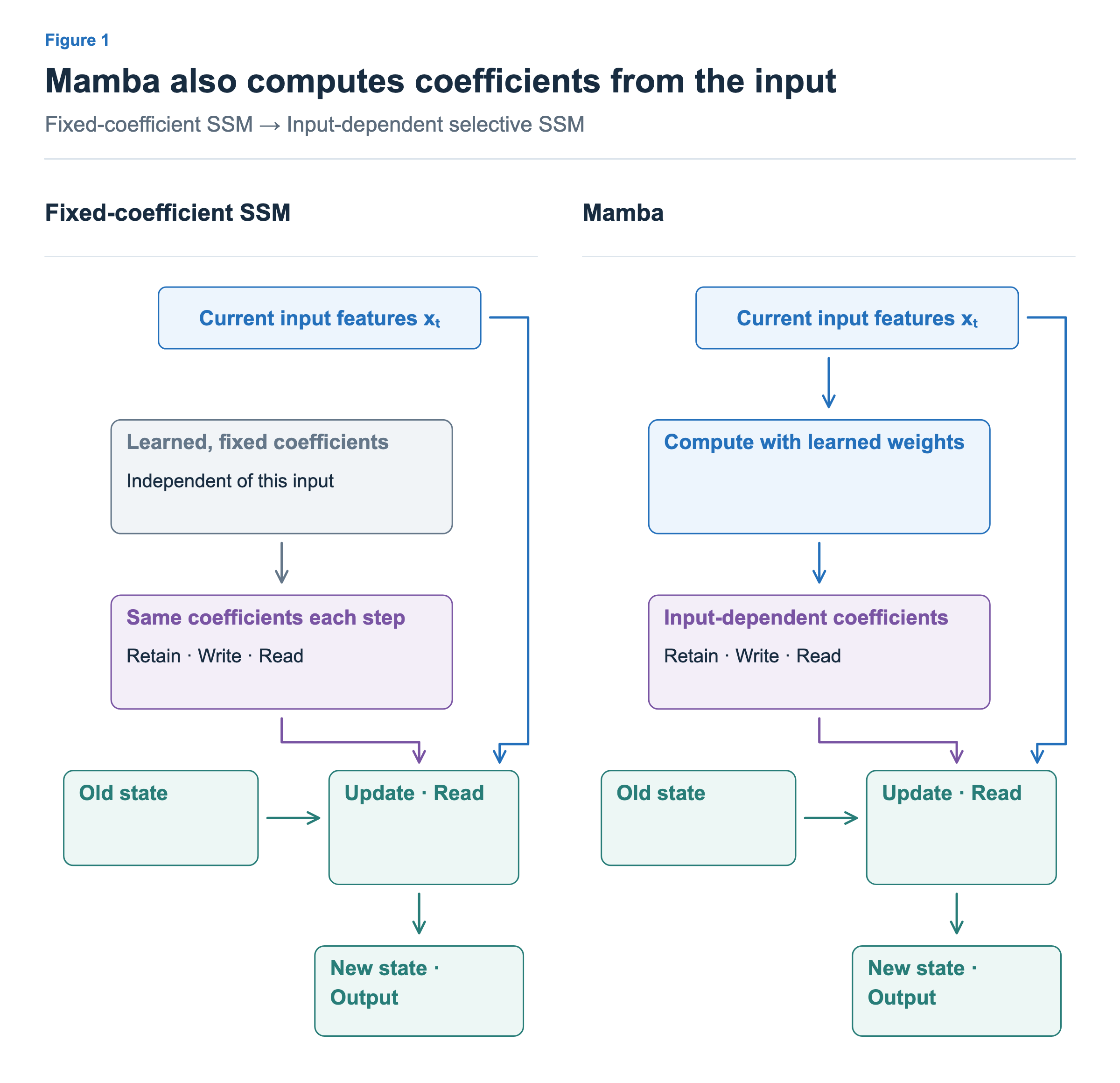
Mamba learns the weights used to compute its coefficients. During inference, these learned weights stay fixed, while the coefficient values are computed from the current input. This works in the same way as using learned weights to produce each token’s Query. Mamba paper §3.1–3.2

Values that control retention, writing, and reading

In the previous article, $\overline{A}$, $\overline{B}$, and C were used directly to update the state and read an output. Mamba computes Δ, B, and C from the input and uses them to construct the coefficients for this step. Let us first examine what changes when each is adjusted.

A and Δ: How much of the previous state remains?

A contains learned rates of change for the state components. In Mamba-1 these values are negative, so the previous state’s contribution decays. Δ is a positive value computed from the input that controls how far that change proceeds in the current step. Think of water cooling at a given rate: less cooling occurs over a short interval and more over a long one. A smaller Δ allows less decay and retains more of the previous state; a larger Δ allows more decay and retains less.

Figure 2 follows just one state component in one channel. The previous state is 2 and A is ln(0.5) in both cases; only Δ changes. With Δ=1, half remains, giving 1. With Δ=2, a quarter remains, giving 0.5.

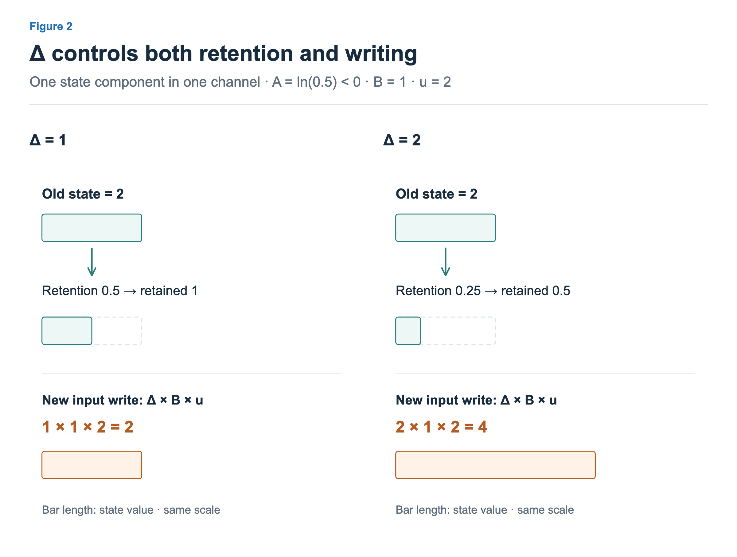
Δ also affects the amount written from the new input. Holding B=1 and input u=2 fixed, the write contribution is 2 for Δ=1 and 4 for Δ=2. With the other values fixed, reducing Δ retains more of the previous state and writes less of the new input.

Mamba computes Δ from the input to adjust retention through A. Generating A itself from each input is also possible, but the paper explains that Δ already makes the effective update coefficients input-dependent, so it keeps A fixed for simplicity. Mamba paper §3.5.2

B: Which components receive the new input?

Although Δ scales the amount written, it cannot freely change the pattern of writing. Suppose one channel has two state components and fixed B=[1, 2]. Increasing Δ from 1 to 2 changes the write coefficients from [1, 2] to [2, 4], but their ratio stays at 1:2.

Computing B from the input can instead produce B=[1, 0] for one input, writing to the first component, and B=[0, 1] for another, writing to the second. Figure 3 uses illustrative values with the same channel input u=1 to isolate this distinction. The two inputs on the right have different full feature vectors, which are assumed to produce different B values.

Computing B directly changes both the amount written and the choice and relative weights of the state components. Changing Δ also changes how much of the previous state is retained. Adjusting B at the same Δ changes the new input’s write contribution without changing that retention.

C: What do we read from the updated state?

C determines how much each state component contributes to the output. For example, C=[1, 0] reads the first component and C=[0, 1] reads the second. Computing C from the input lets the output use components and weights suited to the current input.

A and B govern changes to the state, while C computes the current output from the updated state. C therefore does not require the discretization step that applies the state-update interval Δ.

From input features to update coefficients

We can now put the three paths together. In Figure 4, $x_t$ is the feature vector at the current position entering the SSM. The scalar input u from the previous article is one channel of this vector. The full features generate coefficients, and each channel updates its own state with its own input value. The subscript t marks values computed from the current input.

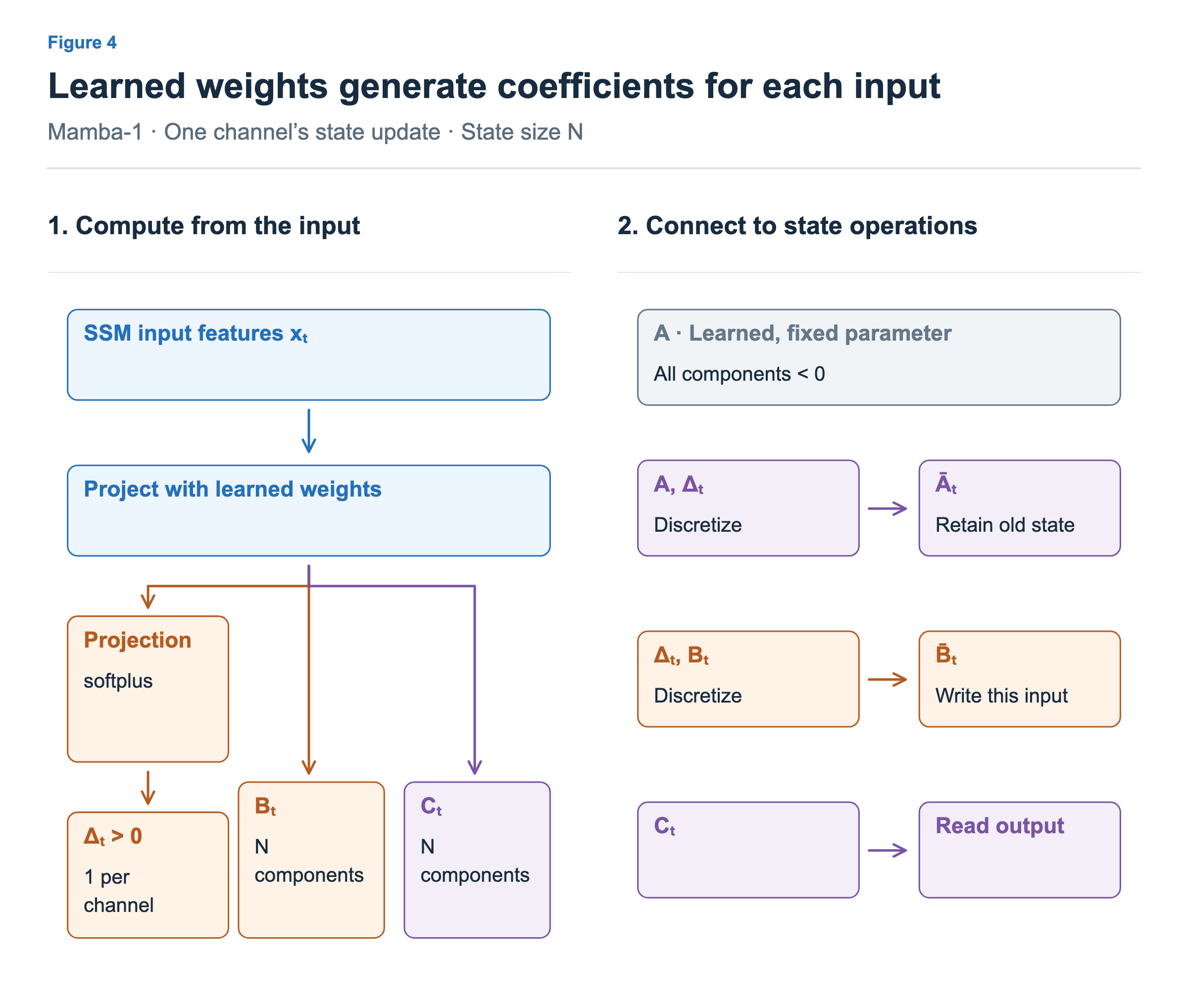
B and C come from projecting the input features with learned weights. With state size N, each has N components; Mamba-1 shares them across channels at the same position. Δ uses a further projection and softplus to produce one positive value per channel. Fixed A and Δ produce the retention coefficients $\overline{A}$; B and Δ produce the write coefficients $\overline{B}$.

Two updates with different coefficients

Let us see how changing the coefficients changes the calculation. Both sides of Figure 5 start from [2, 1]. We assume different full input features produce different coefficients, while keeping the one channel’s scalar input u at 2 in both cases.

The learned A is also the same on both sides. Set its components to ln(0.5) and ln(0.8). Exponentiating them gives 0.5 and 0.8, so Δ=1 yields the same retention coefficients as in the SSM article. These are illustrative coefficients and inputs chosen to make the arithmetic easy to follow.

On the left, Δ=1, B=[1, 0.5], and C=[1, 1]. $\overline{A}$ has components [0.5, 0.8], so the previous state [2, 1] leaves [1, 0.8]. $\overline{B}$=ΔB is [1, 0.5], and multiplying by input 2 gives the write contribution [2, 1]. Adding the contributions produces [3, 1.8], which C reads as 4.8.

On the right, Δ=2, B=[0.25, 0.5], and C=[1, 0]. $\overline{A}$ becomes [0.5², 0.8²]=[0.25, 0.64]. The retained state is [0.5, 0.64]. $\overline{B}$ is 2×[0.25, 0.5]=[0.5, 1], so multiplying by input 2 writes [1, 2]. The new state is [1.5, 2.64].

The final read changes too. C=[1, 0] on the right reads only the first component, producing 1.5. The second component, 2.64, has not disappeared. It does not contribute to this output, but remains in the state for the next input.

Expressing the update and read as equations

Both examples retain part of the previous state, add the current input’s contribution, and read an output. Using the same notation as the SSM article gives the following equations. Here hₜ is the state before processing the current input, hₜ₊₁ is the state afterward, and uₜ and yₜ are one channel’s input and output at the current position.

$$h_{t+1}={\overline{A}}_t{h}_t+{\overline{B}}_t{u}_t$$ $$y_t=C_t{h}_{t+1}$$

The change from the previous SSM equations is the t attached to $\overline{A}$, $\overline{B}$, and C. Previously we repeatedly used the same coefficients; now the current input determines the coefficients used to update and read the state.

The first term is the past contribution retained with the current coefficients; the second is the input contribution written now. These equations show only the state-mediated output. They do not yet include the direct input-to-output path or the output gate covered in the next section.

To make the connection more concrete, the official Mamba-1 single-step implementation constructs the coefficients as follows. A contains the diagonal state-transition components for each channel, and exp acts elementwise.

$${\overline{A}}_t=\exp \left({\Delta }_{t}A\right)$$ $${\overline{B}}_t={\Delta }_t{B}_t$$

Constructing discrete-step coefficients this way is called discretization. The paper explains discretization starting from a continuous-time SSM; the equations above describe the official implementation path followed by our numerical examples. In particular, how $\overline{B}$ is constructed depends on the discretization choice, so these two equations are not universal definitions for every SSM.

The first equation confirms the retention behavior described earlier. Each component of A is negative, so reducing Δ moves ΔA closer to zero and exp(ΔA) closer to one. Multiplying the previous state by nearly one retains most of its value. For A=ln(0.5) in Figure 2, the multiplier is 0.5 at Δ=1 and 0.25 at Δ=2. The second equation shows that reducing Δ at fixed B also reduces the amount written from the input.

In a continuous-time SSM, Δ is the interval over which one update proceeds. Both the old state’s evolution and the accumulation of input occur during that interval, so it enters both update coefficients. A design could instead generate the effective write coefficients directly from the input and control retention and writing separately. Mamba-1 uses Δ in both paths, while input-dependent B provides additional control over the components and proportions written.

Where the state computation sits in a Mamba block

The selective SSM we have examined is the core computation in a Mamba block. The full block also creates the features entering the SSM and processes its readout into an output. Figure 6 locates these operations in a representative Mamba-1 block.

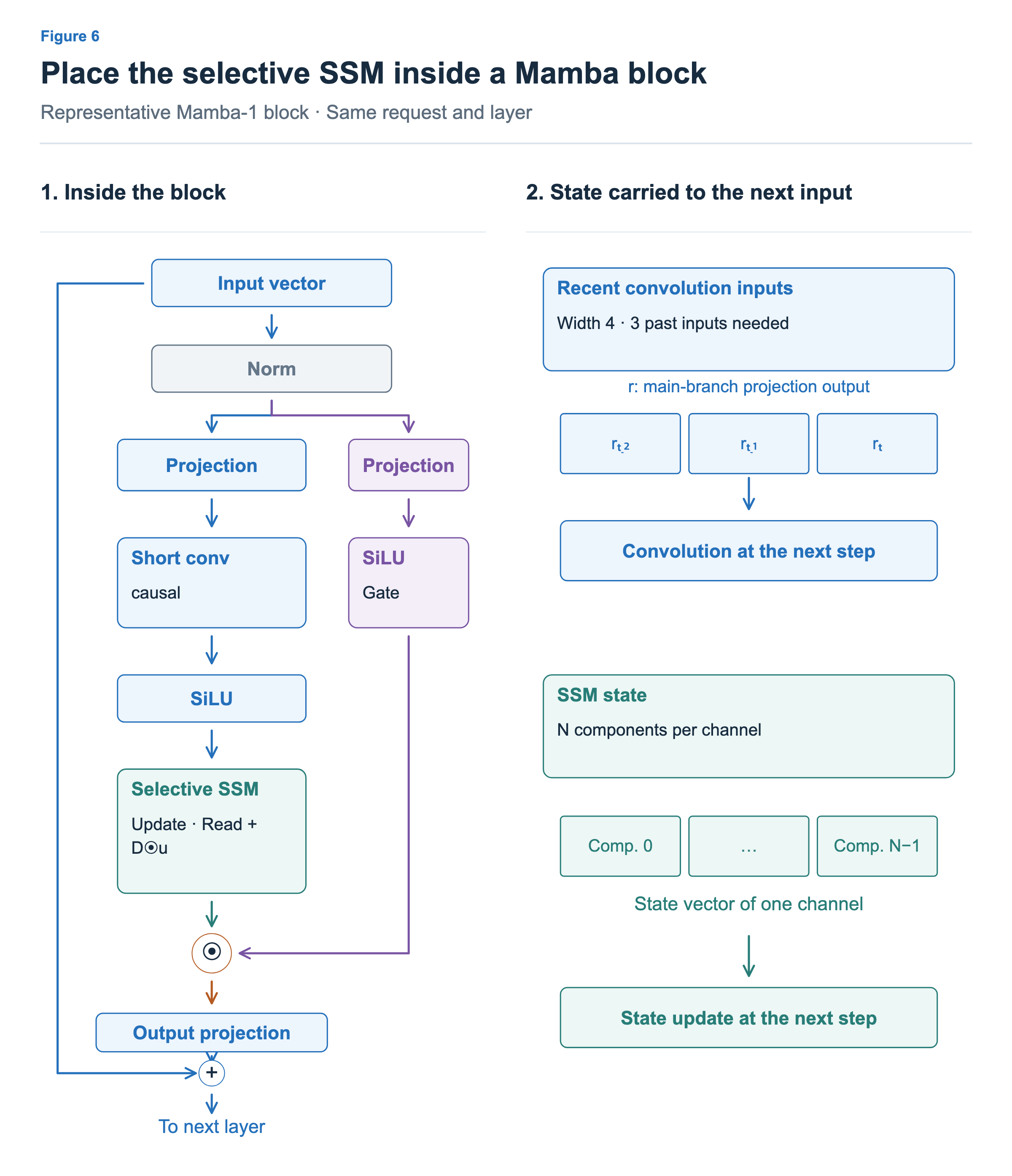
The input vector passes through normalization and projection and splits into two branches. The main branch uses a short causal convolution, which processes the current position together with nearby past inputs. A SiLU activation follows, and the resulting features enter the selective SSM. These are the input features we called x above.

The selective SSM updates and reads the state. The actual computation also includes D⊙u, a term adding the current input directly to the output. D is a learned per-channel weight.

The other branch applies SiLU and multiplies the main branch’s result elementwise. This output gate adjusts an already computed output. It acts at a different point from Δ, which controls the state update. Because it uses SiLU, it cannot be interpreted as a retention rate always between 0 and 1. An output projection follows, and the result is added to the block’s residual input before reaching the next layer. Mamba paper §3.4

Two kinds of state remain for the next token. The convolution needs recent input history. With width 4, it needs three past values alongside the next input.

The SSM retains N state components per channel. If a layer has $d_{\text{inner}}$ internal channels, its SSM state for one request contains $d_{\text{inner}}\times N$ components. Convolution history is separate. With model size and convolution width fixed, neither state grows continually with the number of generated tokens. This differs from attention’s addition of KV for each past token. State allocation in the official implementation

Comparing Mamba with delta corrections in GDN and KDA

Mamba, GDN, and KDA all carry a fixed-size state and compute values from the current input to control it. Saying that they “adjust memory based on the input” is therefore insufficient to distinguish them. We need to compare how they construct the contribution added to the retained state.

GDN and KDA read the retained state with the current Key, then subtract that readout from the current Value. To revise what is associated with this Key, they first check what is already associated with it. Mamba computes a contribution from the current input and adds it to the state without this Key lookup and difference calculation.

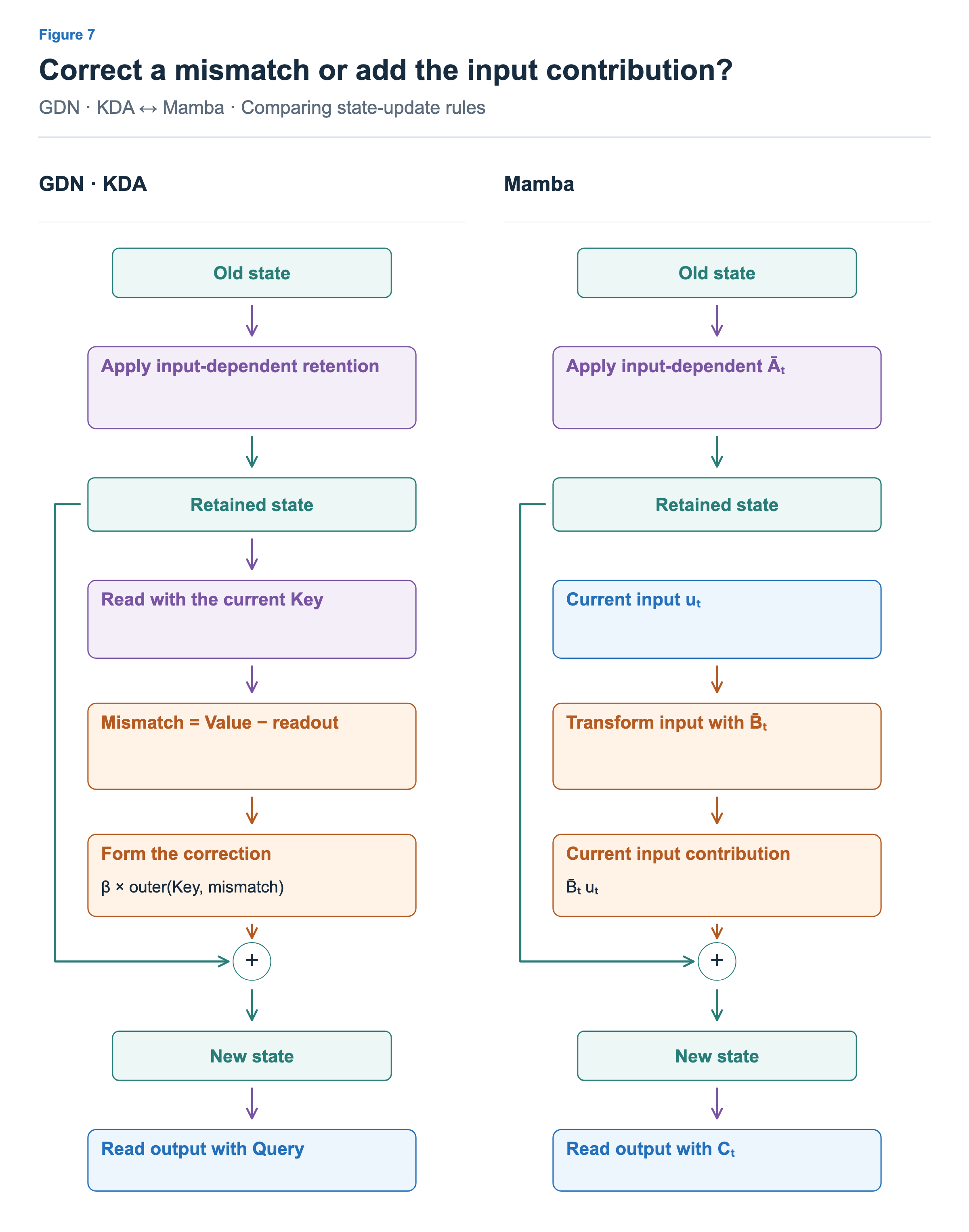
On the left, the correction depends on both the new Value and the existing state’s readout. Even with the same Key and Value, the needed correction varies with what is already remembered. If the readout already equals the new Value, the difference is zero, leaving no delta correction to add. Gated DeltaNet paper §2–3, Kimi Linear paper §3

On the right, Mamba computes its write contribution from the current SSM input and the input-derived $\overline{B}$. Identical SSM input features give the same write contribution; a different previous state changes the past contribution produced by $\overline{A}$. Both approaches subsequently read an output from the updated state.