Hybrid Models: Using State and Attention Together

The models covered from Linear Attention through Mamba preserve the influence of past inputs in a state. Each new token updates that state, then reads the values needed for its current output. Once the model’s state size is fixed, generating more tokens does not continually increase this storage.

Should we therefore replace every Attention layer with a state-based layer? That is a natural choice if reducing storage is the only objective. But it also changes how the model uses past information. Reading what has been written into a state differs from retaining KV at past positions and referring to it again with the current Query.

This article examines hybrid models that place these two computations in different layers. We will first consider why to combine them and the potential quality benefits, then examine the remaining memory and execution costs. Finally, we will follow one token through a state-based layer and an Attention layer.

Memory in a state and memory indexed by position

First, compare what each approach stores. Both sides of Figure 1 receive the same four positions p₀, p₁, p₂, and p₃. Each position block represents one vector entering that layer. A small cell inside the state represents a state component, not a vector.

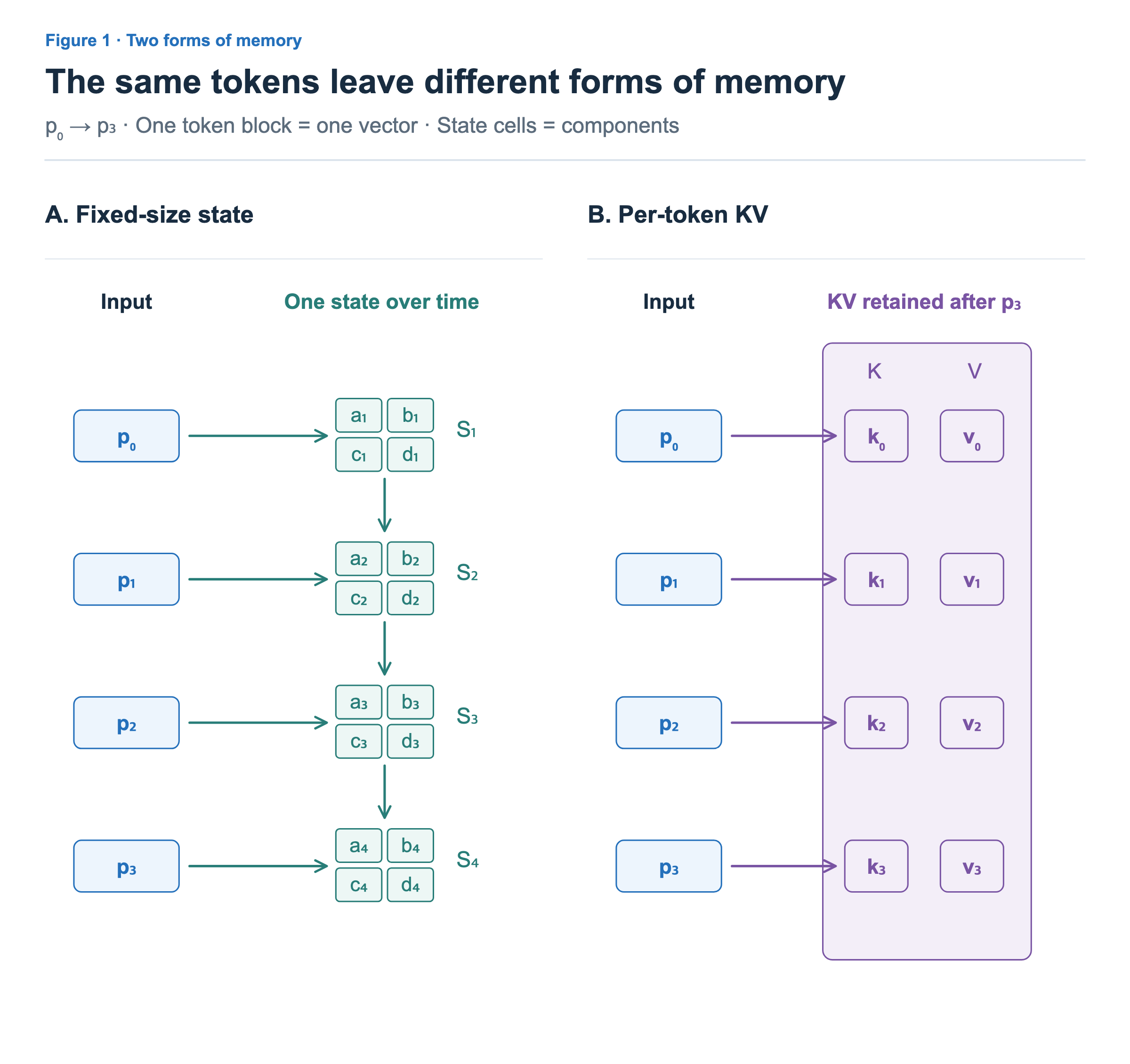
The left side updates a state of the same size whenever an input arrives. The figure shows several states to display its change over time; generation does not retain all these snapshots. After processing p₃, the final state is passed on to the next token.

The right side retains the Key and Value produced at each position. After p₃, it stores four positions’ KV. The next position’s Query can score these positions separately and read their Values with the resulting weights. KV here is not the original text tokens themselves, but representations computed in that layer.

In a state-based layer, multiple records affect the same components, and updates can change earlier records. KV Attention retains representations by position, allowing the current Query to compare those positions again.

Placing the two computations in different layers

State-based computation repeatedly updates context. GDN and KDA incorporate the difference between the existing state’s readout and the new Value, while Mamba adjusts retention, writing, and reading coefficients based on the input. These updates are a way of processing information as well as saving storage.

KV Attention provides a path that directly compares representations at past positions using the current Query. A hybrid model can preserve this path in some layers and update state in others. Figure 2 is an educational example that keeps the total at six layers and compares their arrangement.

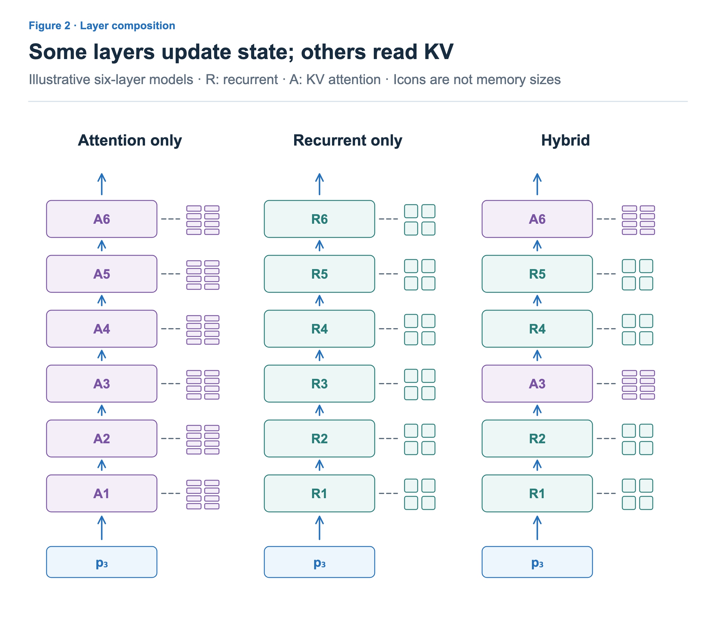
The middle configuration uses state in every layer. The hybrid on the right processes R₁ → R₂ → A₃ → R₄ → R₅ → A₆. R denotes a state-based layer, A a KV Attention layer, and each subscript is a layer number. Each R layer has its own state, and A₃ and A₆ each store their own KV.

The same token’s representation passes through every layer in sequence. A state-based layer’s output becomes the next Attention layer’s input; the result of consulting past positions in Attention then passes to later state-based layers. The two computations are connected through depth.

Can combining them also improve quality?

Combining the two approaches is not only about accepting a quality loss to save memory. Some experiments find that a hybrid model outperforms either individual type under the same training conditions.

Figure 3 shows a comparison from the Mamba-2 paper. Models with approximately 350M parameters were trained on 7B Pile tokens and compared using the same GPT-2 tokenizer and training and validation conditions. Perplexity evaluates next-token prediction; lower is better in this comparison.

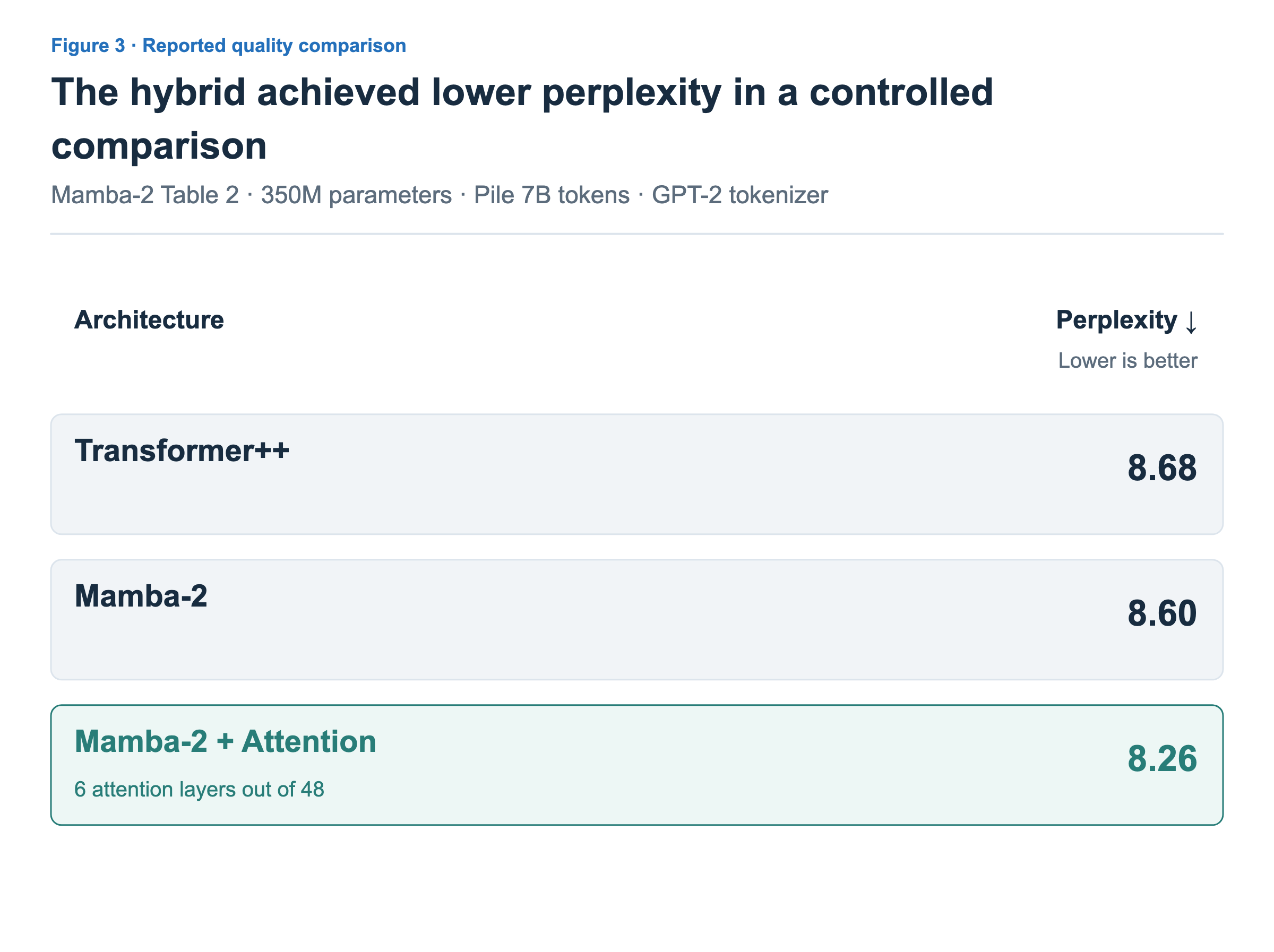
Transformer++ scores 8.68 and Mamba-2 scores 8.60, while a hybrid with Attention in 6 of Mamba-2’s 48 layers scores 8.26. In this experiment, the hybrid achieves lower perplexity than either the Attention-only or state-only configuration. Mamba-2 paper §9.2.3, Table 2

This result shows that combining the two computations can improve prediction quality. The appropriate layer ratio depends on model scale and training conditions.

Reduced storage and remaining costs

In a hybrid model, the cache in KV layers still grows with context length. Figure 4 returns to the six-layer example and compares storage after four and eight tokens. This storage calculation is separate from the experimental model in Figure 3.

Assume each state-based layer stores a 2×2 state, or four components. Each Attention layer stores two Key components and two Value components per token. Every cell represents one component of equal size, not a head or a whole token.

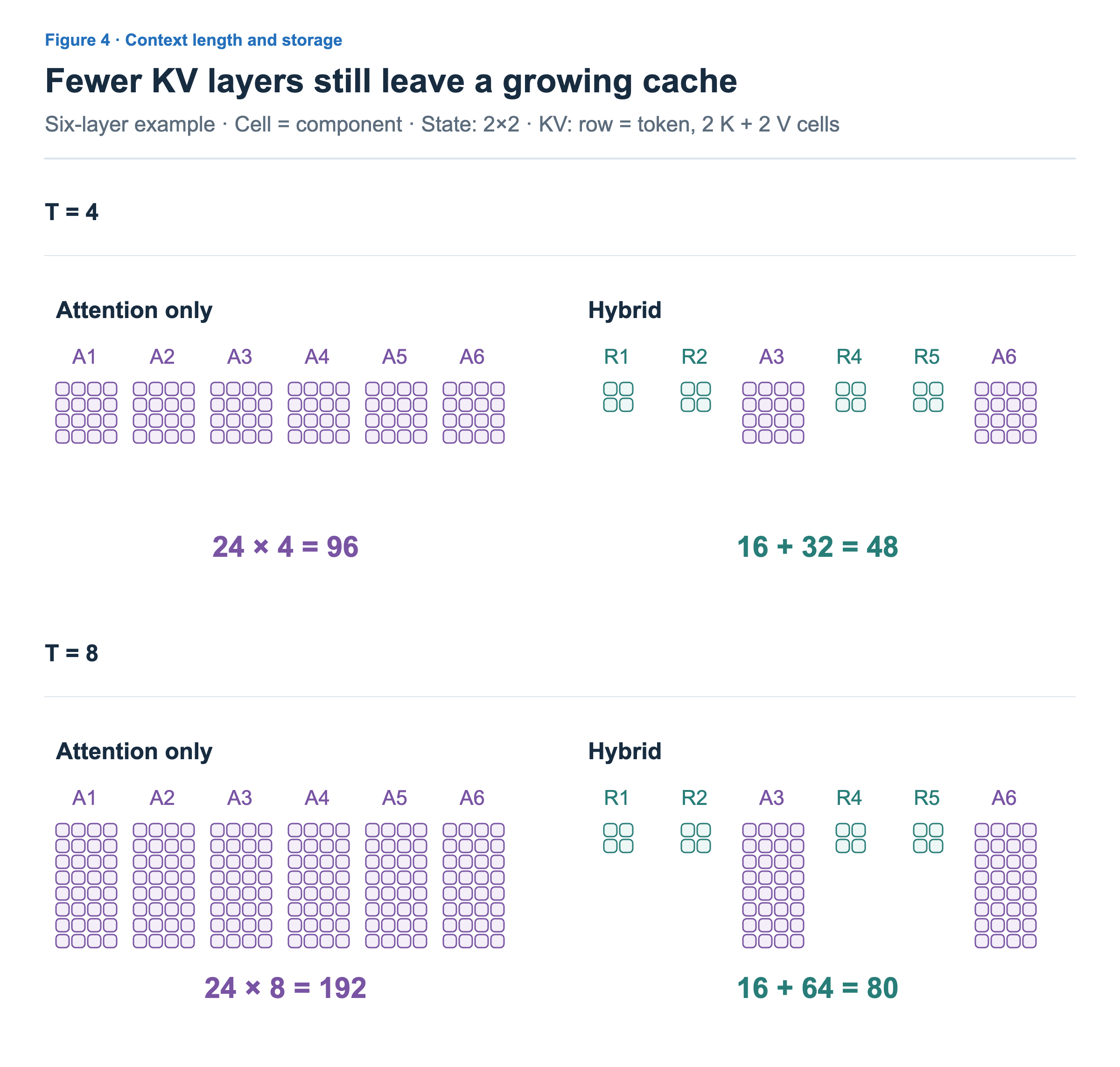
If all layers use Attention, each layer needs four times the token count in components. Across six layers, the total is 24T for T tokens: 96 at T=4 and 192 at T=8.

In the hybrid, the four state layers remain at 16 components in total. The two Attention layers store 8T components. Total storage is therefore 16+8T: 48 at T=4 and 80 at T=8. Fewer KV layers reduce the rate of growth, but total storage is not fixed.

This calculation compares only state and KV storage, excluding weights, intermediate activations, and other memory use. Fixed-size states also require storage, so the benefit may be smaller at short context lengths.

Quality and execution bring further considerations. Reducing Attention layers also reduces the number of stages that directly refer to position-indexed KV. Training and evaluation must establish whether the remaining stages preserve the needed quality.

The runtime must also manage two forms of memory. KV appends a row for each new position, whereas state updates existing contents. For example, after processing a candidate continuation, returning to an earlier position can discard appended KV rows. Recovering an overwritten state requires a saved earlier value or a way to recompute it. This is an execution difference to consider separately from layer ratios. How much reduced KV access improves actual speed also depends on state-update kernels, context length, and batch size.

Different hybrids combine different things

The name Hybrid Attention does not always refer to the state-and-KV combination discussed so far. It can also describe arrangements of SWA or compressed Attention across layers. Figure 5 distinguishes them by what is being combined.

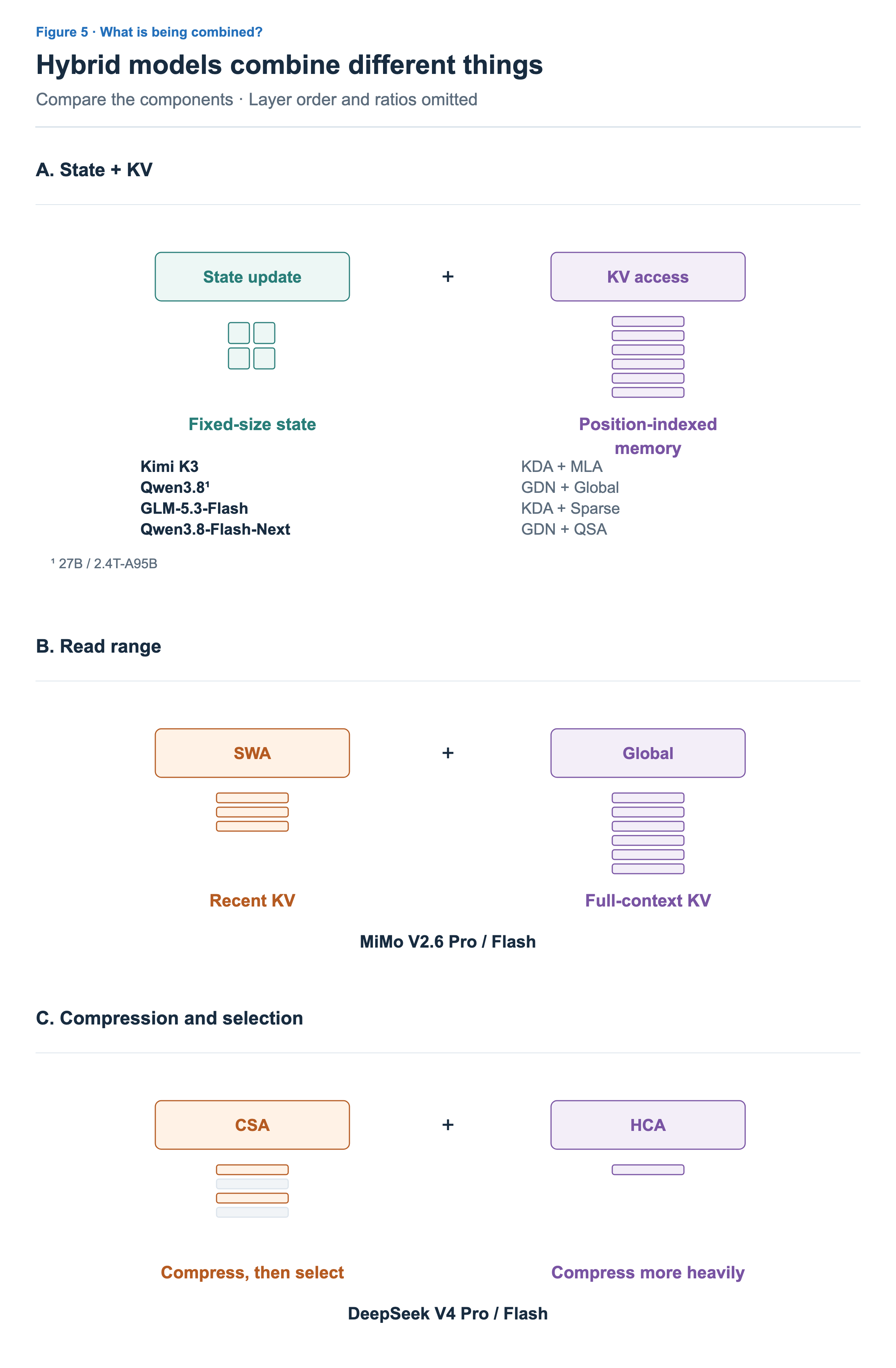
The first type, central to this article, combines state-based layers with KV Attention layers. Kimi K3 uses KDA and MLA; Qwen3.8-27B uses GDN and full-context Attention. The KV side need not be conventional Full Attention. GLM-5.3-Flash combines KDA and Sparse Attention, while Qwen3.8-Flash-Next combines GDN and QSA.

The second type combines KV read ranges. Models such as MiMo-V2.6-Pro-RL place recent-window SWA alongside full-context Attention. SWA stores and reads position-indexed KV within a recent window.

The third type combines compression and selection methods. DeepSeek-V4 uses CSA, which compresses multiple tokens’ KV and selects some entries, alongside more heavily compressed HCA. Both also include a path that reads uncompressed recent-window KV. Compressed entries are KV added as the number of token groups increases; this differs from repeatedly updating a single state of fixed size.

Following one token through both types of layers

Finally, follow p₃ through the hybrid configuration in Figure 2. Let layer 2 use GDN and layer 3 use KV Attention. Both layers hold memory from processing p₀ through p₂ and now receive an input representation for p₃.

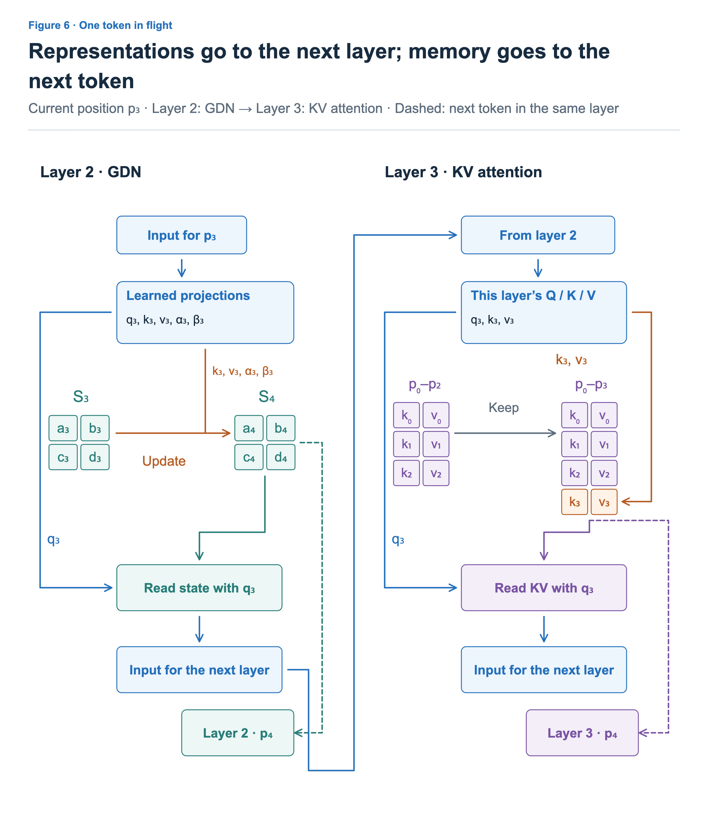
Layer 2 first uses learned weights to derive a Query, Key, Value, retention factor α₃, and correction strength β₃ from its input representation.

It then applies retention to the existing state S₃ and reads the retained state with k₃. The difference between the Value to write, v₃, and this readout is combined with β₃ and k₃ to form a correction and update the state. This is the GDN computation covered earlier.

The updated state is S₄. As in the earlier articles, the state subscript counts processed tokens, so S₃ precedes processing p₃ and S₄ follows it. The current q₃ reads this new state to produce an output for the current position. The representation passes through the remaining block operations, such as output projection, residual connections, and FFN, and becomes the next layer’s input.

Layer 3 uses its own weights to compute a new Query, Key, and Value from the received representation. Both panels use the symbols q₃, k₃, and v₃, but these are different vectors because they belong to different layers. Subscript 3 denotes the current token position; the panel title identifies the layer.

Layer 3’s cache holds KV for p₀ through p₂. It appends its own k₃ and v₃, then uses q₃ to read KV from p₀ through p₃. The resulting output becomes the next layer’s input representation. Layer 2’s state is neither converted into KV nor copied into layer 3’s cache.

When p₄ arrives, layer 2 continues by updating its own S₄, while layer 3 keeps its own four positions’ KV and appends a new row. The current token’s representation flows to the next layer; each layer’s memory carries forward to the next token in that same layer.