HC and mHC: Widening and Connecting Residual Streams

In Residual Connections and RMSNorm, the basic connection added the result of the current computation to the previous representation. When attention or an MLP produces new information, that result accumulates in the same vector and passes to the next computation.

So far, this advanced model series has focused mainly on reading information across tokens and storing context. We now turn to how the representation of the same token travels through model depth. Hyper-Connections (HC) maintain several streams for carrying results and learn the connections that read and update them. We then examine why mHC constrains one of those connections: the bypass mixing path.

Layer outputs accumulating in one vector

A stream here is a path that carries a token’s representation from one layer to the next. Let e be the input embedding, $f_{1}$ the fresh output of the first computation, and $f_{2}$ the fresh output of the second. With a standard residual connection, the representation changes as e → e + $f_{1}$ → e + $f_{1}$ + $f_{2}$ .

The left side of Figure 1 shows this accumulation. The right side shows several representations maintained together for the same token. Moving down the diagram means moving through model depth, not through the token sequence.

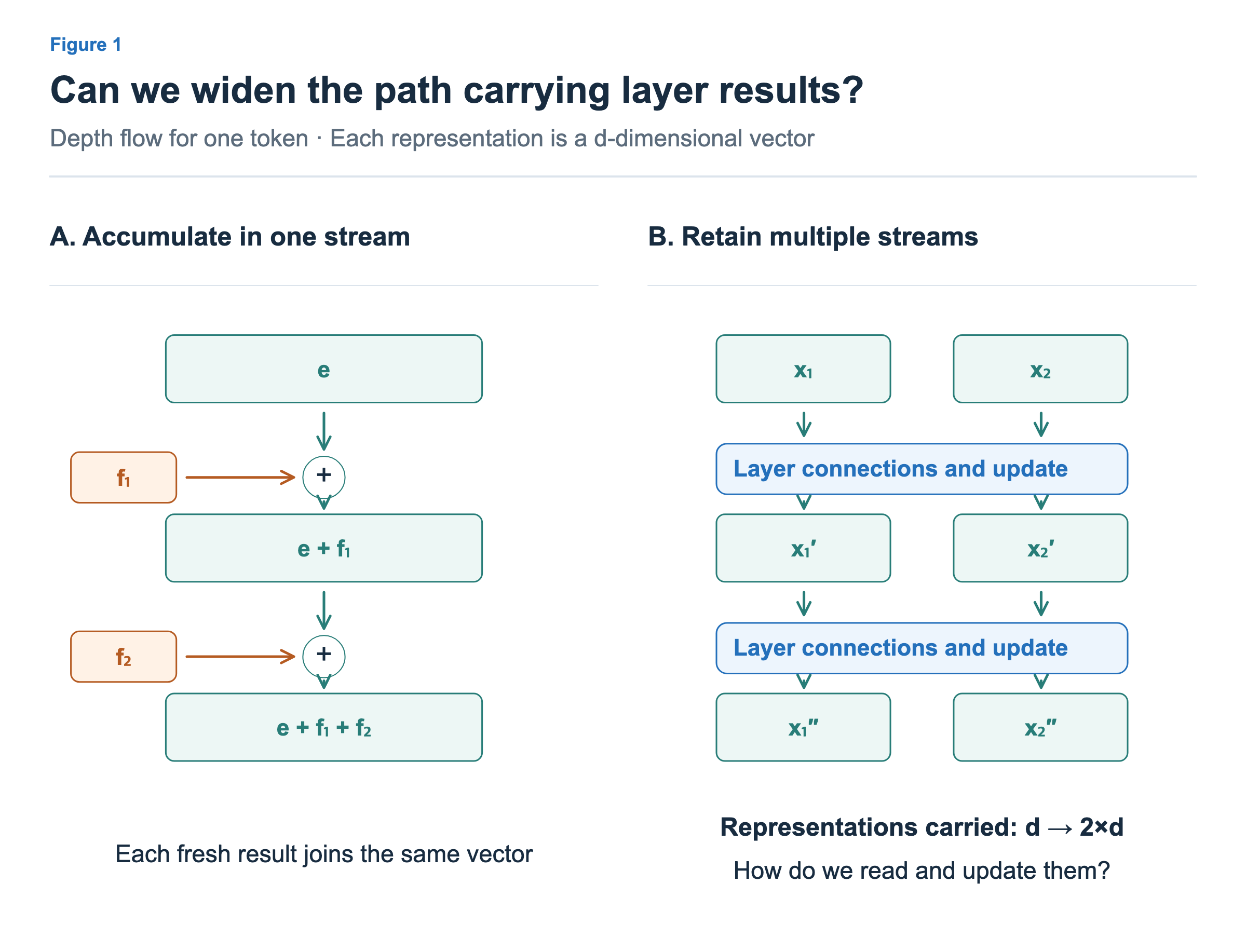
Left: f1 and f2 are added to e, yielding e+f1+f2. Right: two representations of the same token persist at each depth and update through layer connection boxes.

Adding results into one vector does not mean that all earlier information disappears. A trained model can represent the features it needs within that vector. What the next computation receives, however, is an already combined representation. The standard residual connection does not include an operation that retrieves each layer’s contribution separately and assigns it a weight.

Multiple streams allow several d-dimensional representations to coexist at the same point. The two streams in this article hold 2d components in total. Their roles are not prescribed as, for example, grammar in the first stream and meaning in the second. The design gives them room to learn different contents. HC turns this idea into concrete connections.

Reading from and writing to a wider path

Does storing two representations require running attention and the MLP twice? HC first combines multiple streams into one d-dimensional input. A computation block F processes that input, and its d-dimensional output is distributed back to the streams. F represents attention or an MLP; the diagram folds away details such as normalization.

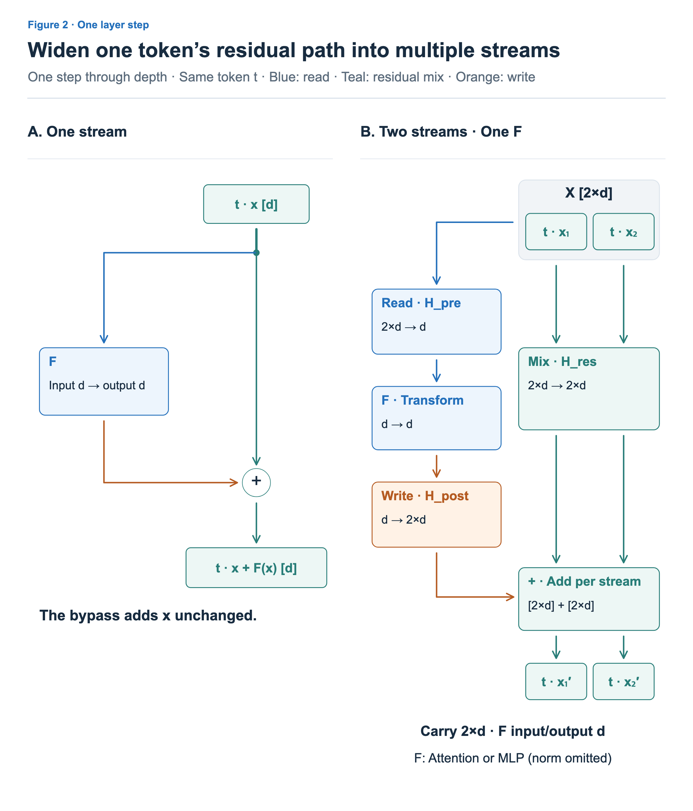
A splits one d-dimensional x for token t between F and a bypass, then adds them. B has two streams x1,x2 for the same token t. Blue read combines them into one d-dimensional F input, orange write distributes its output to 2×d, and a separate teal residual mapping mixes the bypass. The two contributions are added per stream.

The key distinction in Figure 2 is between the width of the representations being carried and the width of F’s input. The residual path with two streams has width 2d, while F’s input and output still have width d. A separate bypass path mixes the two existing streams, and the contribution from F is added to that result.

Section 3 of the mHC paper, which describes HC, separates these connections into read $H_{pre}$ , bypass mixing $H_{res}$ , and write $H_{post}$ mappings. The parameters that produce the coefficients are learned, and dynamic connections also let the coefficients depend on the current representation. The numbers below are illustrative coefficients chosen for one computation point.

Two paths from the same input

Let the two streams be $x_{1}$ = [2, 0] and $x_{2}$ = [0, 2]. Stacking them as rows gives a 2×2 matrix X. Rows identify streams, and columns identify vector components. The two sizes happen to be equal in this example, but stream count and feature dimension d are different axes.

The left side of Figure 3 takes X through the path that produces F’s input and the write contributions. The right side is a bypass path starting from the same X. Its mixing operation does not take the read result on the left as its input.

H_pre [.75,.25] reads X=[[2,0],[0,2]] as [1.5,.5], with assumed F output [.4,−.2]. H_res=[[.8,.2],[.2,.8]] mixes the same X into B=[[1.6,.4],[.4,1.6]]. The write column [1,.5] times u gives W=[[.4,−.2],[.2,−.1]], and B+W produces [[2,.2],[.6,1.5]].

With read coefficients 0.75 and 0.25, the input to F is:

0.75 x_{1} + 0.25 x_{2} = [1.5, 0.5]

We omit F’s internal computation and assume an output u = [0.4, −0.2]. The first stream receives 1 times u, and the second receives 0.5 times u. The contributions to add are therefore [0.4, −0.2] and [0.2, −0.1]. A write coefficient is a scalar applied to the entire vector sent to one stream.

On the bypass path, the first stream combines 0.8 times the original $x_{1}$ and 0.2 times $x_{2}$ , producing [1.6, 0.4]. The second reverses those proportions to produce [0.4, 1.6]. Finally, the two paths are added together.

Stream	Bypass result B	Fresh write contribution W	Next representation B + W
First	[1.6, 0.4]	[0.4, −0.2]	[2, 0.2]
Second	[0.4, 1.6]	[0.2, −0.1]	[0.6, 1.5]

The read determines what F sees, bypass mixing determines how existing representations pass onward, and the write determines where and how much of the fresh result is added. All three can be described as weighted combinations, but their inputs, outputs, and roles differ.

For n streams, X has shape n×d, the read matrix has shape 1×n, and bypass mixing has shape n×n. This article represents the write coefficients as an n×1 column vector, so multiplying them by F’s 1×d output produces an n×d write contribution. The figure’s $H_{post}$ is the transpose of the row-vector convention in the original paper. The fact that the example read coefficients sum to one does not imply that all HC read and write coefficients must do so.

When mixing repeats through depth

The bypass in a standard residual connection passes its input through unchanged. If F outputs zero, the next representation equals the previous one. HC also has a mixing matrix on the bypass, so existing representations can change even when F contributes no new value.

Figure 4 sets all F outputs to zero to isolate this effect. Here, [2, 0] contains one corresponding component from each of the two streams. Its axis differs from the previous section, where a vector listed two components of one stream.

Identity keeps [2,0]. Left 2I yields [2,0], [4,0], [8,0], [16,0]. Right H=[[.8,.2],[.2,.8]] yields [2,0], [1.6,.4], [1.36,.64], [1.216,.784], retaining sum 2.

With the identity matrix I, [2, 0] remains [2, 0]. Repeatedly applying 2I instead produces [4, 0], [8, 0], and [16, 0]. Values grow along the bypass even without adding new information. This is an example permitted by unconstrained connections, not a prediction that HC must learn this behavior.

The 0.8/0.2 mixing on the right changes [2, 0] into [1.6, 0.4], [1.36, 0.64], and [1.216, 0.784]. The values mix, but their sum remains 2 at every step. mHC constrains bypass mixing to have this kind of conservation property.

What mHC preserves

mHC targets a bypass mixing matrix with nonnegative entries and row and column sums of one. Such a matrix is called doubly stochastic. Figure 5 uses the same [2, 0] example to show what the row and column conditions mean.

Mixing [2,0] gives [1.6,.4], both within0–2 and summing to2. H_res=[[.8,.2],[.2,.8]] has unit row and column sums, obtained from positive scores by iterative normalization.

When a row sums to one, its output is a proportional mixture of the inputs. For example, 0.8×2 + 0.2×0 = 1.6. Because this is an average with nonnegative weights, the result lies between the input minimum, 0, and maximum, 2. When a column sums to one, the total scale with which one input is distributed across outputs is one. The sum of all outputs therefore equals the sum of all inputs.

A product of these matrices has the same properties. That is why repeated mixing in the previous figure did not push values outside the initial range of [2, 0]. Preserving the sum does not preserve each stream’s contents unchanged, however. The example also shows the two values moving closer together as mixing repeats.

Section 4 of the mHC paper uses the Sinkhorn-Knopp procedure, which repeatedly normalizes rows and columns of scores transformed to positive values. A finite number of iterations approximates the constraint, and the read and write coefficients use separate transformations. Not every connection matrix is made doubly stochastic.

This conservation property also concerns bypass mixing before adding the fresh F output. It does not mean that the magnitude of the entire representation, including F’s write contribution, is fixed, or that all sources of training instability disappear.

Representation capacity and execution cost

HC creates room to maintain several representations on the residual path, while mHC constrains the mixing used to connect that path repeatedly. The aim is to use richer connections while reducing the risk of excessive amplification along the bypass.

Keeping F’s width at d does not leave the total cost unchanged. Carrying, reading, and writing n representations increases activation storage and memory traffic. Producing connection coefficients and mixing streams adds computation as well. At the same token count and d, the residual representations themselves contain n times as many components, but total model memory or runtime does not automatically grow by that factor. Other costs, including attention’s KV cache, MLP intermediates, and kernel organization, contribute too.

The quantities to check therefore include training stability, activation memory, and actual runtime as well as accuracy. The small numerical examples in this article explain the connections; they are not measurements of performance improvements.

The next article on Gated Residual also maintains multiple streams. It keeps the originals on the bypass, however, and applies gates to individual vector components during the read. We move from what is stored to how the stored representations are used.