Gated Residual: Reading Components and Writing to Originals

HC and mHC stored several representations of the same token in multiple streams. Each computation reads those representations to form one input and writes its fresh output back to the streams. mHC separately constrained the bypass path that mixes existing streams.

Gated Residual (GR) also maintains multiple representations. What changes is how it controls the read for each vector component and adds fresh results to the original representations. Interpreting a gate as removing a fraction of the previous representation can easily confuse the read and write paths. We will separate those paths, then follow one numerical example through to the end.

Here, GR means the design in Section 2.2 of the Qwen3.8-Flash-Next report. We will not treat every similarly named gated residual variant as the same rule. The report uses four branches; the figures reduce this to two to make the calculation easier to follow. A branch here is the path that carries a representation of the same token, called a stream in the previous article.

Bypass and read paths

In Figure 1, both mHC and GR combine multiple representations into one input to F, then send F’s output back to the paths. F is attention or an MLP. Start by following the bypass that carries an original representation into the next one.

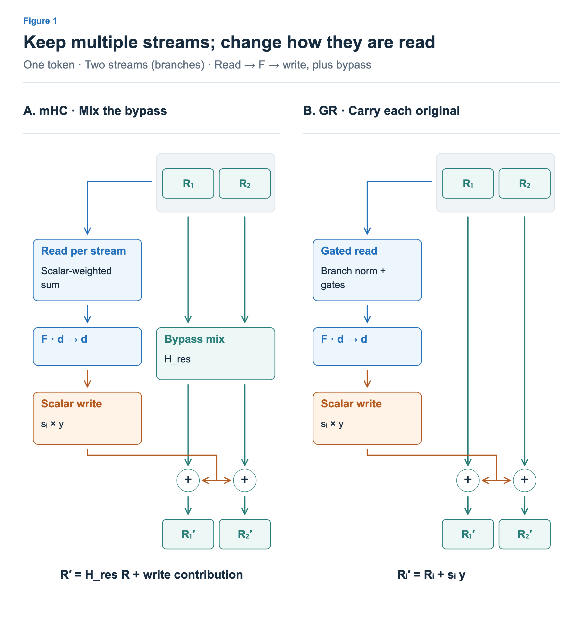
In mHC, $H_{\text{res}}$ on the bypass mixes the existing streams. GR’s bypass passes each original branch through unchanged. The newly computed value is added to that original. This GR therefore has no direct branch mixing corresponding to mHC’s bypass mixing matrix.

That does not make the branches independent models. The read uses information from multiple branches together, and several branches receive the result of a shared F. Directly mixing bypass paths is different from interaction through reading and computation.

The read also differs. In the previous article, mHC multiplied each stream by one scalar. GR normalizes each branch and multiplies individual components by different gates. It can read some components of the same branch more strongly than others.

Normalizing and reading each branch

Let the originals be $R_1$ = [2, 2] and $R_2$ = [4, −4]. Figure 2 shows two uses for their normalized values: one path supplies the values to read, while the other feeds the controller that computes the read gates.

First, apply RMSNorm separately to each branch. To simplify the calculation, set the learned gain to one and omit the small stabilizing constant ε. The RMS of [2, 2] is √((4 + 4) / 2) = 2, so dividing gives [1, 1]. The RMS of [4, −4] is 4, giving [1, −1]. Normalization does not merge the two branches into one.

A hat over R in the figure denotes a normalized value. Subsequent reads use these values, but the originals [2, 2] and [4, −4] continue along the bypass in the preceding figure. The originals are also where the fresh output will be added later.

The controller sees all normalized branches together and produces a gate for each branch and component. It is a learned transformation that computes coefficients for each input, not a process that retrains controller weights during inference. The internal projections in Equation (31) of the report are folded into the controller box.

Suppose the gates for this input are $G_1$ = [0.8, 0.2] and $G_2$ = [0.4, 0.6]. These are illustrative controller outputs. They cannot be calculated from the two originals alone without the controller’s weights.

Branch	Normalized value	Componentwise gate	Componentwise product
First	[1, 1]	[0.8, 0.2]	[0.8, 0.2]
Second	[1, −1]	[0.4, 0.6]	[0.4, −0.6]

The figure uses ⊙ for componentwise multiplication. The first component of the first branch is scaled by 0.8 and its second component by 0.2. This controls the read more finely than multiplying the entire vector by one scalar.

Next, add the two results and divide by the branch count, two.

$$x=\frac{[0.8,0.2]+[0.4,-0.6]}{2}=[0.6,-0.2]$$

This x goes into F. For n branches, the same procedure sums their gated values and divides by n. The divisor is not the sum of the gates. In this example, the gates sum to 1.2 for the first component and 0.8 for the second, but both components are divided by the branch count of two.

The read gates come from a sigmoid, without a softmax that makes them sum to one across branches. It is therefore more accurate to interpret them as scales for normalized components than as probabilities of selecting the two branches. A small gate means that a component contributes less to F’s input, not that the component has been deleted from the original.

Writing fresh output to the originals

Suppose F receives the read result x = [0.6, −0.2] and produces a fresh output y = [0.5, −0.25]. This example does not expand F’s internal computation. We now decide how much of y to add to each original.

In Figure 3, a write controller separate from the read gates produces one scalar per branch. This controller also receives all normalized branches as input.

In Equations (33)–(34) of the report, the write coefficients are twice a sigmoid output and therefore lie between zero and two. Let $s_1$ = 1.2 and $s_2$ = 0.4 for this example. The read used different gates for different components, but the write multiplies every component of y sent to one branch by the same scalar.

The first branch receives 1.2×[0.5, −0.25] = [0.6, −0.3]. The second receives 0.4×[0.5, −0.25] = [0.2, −0.1]. Adding these contributions to the originals gives:

Branch	Preserved original	Scaled fresh output	Next branch
First	[2, 2]	[0.6, −0.3]	[2.6, 1.7]
Second	[4, −4]	[0.2, −0.1]	[4.2, −4.1]

Let $R_i$ be the original value of branch i and $s_i$ its write scale. The update fits in one line:

$$R_i^{\prime }=R_i+s_{i}y$$

The scale multiplies the fresh output y. It does not multiply the original $R_i$. A small $s_i$ therefore means a smaller fresh contribution added to the original, rather than retaining only a small portion of that original. In the limiting case as the scale approaches zero, the branch passes onward a value close to its original.

A positive scale does not mean that every component increases. In the example, the second component of the first branch decreases from 2 to 1.7 because the added contribution is −0.3. The signs of both the coefficient and the vector components matter.

Distinguishing gates from retention

In GDN and KDA, a retention factor multiplied the existing state when a token arrived. That operation determined how much of the previous state itself remained. GR’s bypass here has no such decay.

Control	Where the scale is applied	What changes directly
State retention	Previous state	Existing state retained at the next step
GR read gate	Each normalized branch component	Input to the current F
GR write scalar	F’s fresh output	New contribution added to the original branch

The earlier state updates also followed the token sequence, while this residual propagation follows model depth. The word “gate” can refer to different quantities and axes.

The cost and purpose of finer reads

GR combines the capacity of multiple representations with flexibility in deciding what to read from them. It can scale individual components within one branch differently while carrying the original unchanged on the bypass. Rather than summarizing it only as “how much information passes from the previous layer,” it helps to separate what is read for the current computation from how much of its result is written.

Storage and memory traffic remain because multiple branches are maintained. Branchwise normalization and the gate controller also require computation. Removing the bypass mixing matrix alone does not establish that GR is faster than mHC in every setting. Cost must be checked for the branch count, dimension, kernel organization, and phase of training or inference.

The report’s stability discussion relies on separate comparison experiments in Section 3.3. Reducing a value with a gate in this numerical example does not prove stability for the entire model. A calculation that explains the structure and an actual training result are different kinds of evidence.

The next article on Attention Residuals changes the storage scheme. Instead of repeatedly updating a few branches, it retains fresh outputs from earlier layers and computes how much of each the next layer should read.