Attention Residuals: Selecting Outputs from Earlier Layers

HC/mHC and Gated Residual maintained representations of the same token in multiple streams. Each layer read those representations, computed a result, and wrote it back to the streams. They did not retain a separate output from every earlier layer.

Attention Residuals (AttnRes) starts with a different question: can we keep earlier layers’ results separate and let the next layer choose what to read? It applies the idea of attention, which selects information across tokens, to connections along depth.

We first examine the Full form, which stores individual outputs, and its weighted read. We then connect that read to the computation of its weights. Finally, we consider the trade-off in the Block form, which groups outputs for storage, and compare it with the previous two families. The specific scoring and block definitions follow Section 2.2 of the Kimi K3 report.

Accumulated representations and individual outputs

Let e be the embedding, and $f_1$ and $f_2$ the fresh outputs of successive sublayers. A sublayer here is a computation with a residual connection, such as attention or an MLP. Subscripts in the figures identify computation depth, not token position.

A standard residual connection passes the combined representation of e, $f_1$, and $f_2$ into the next F. Full AttnRes stores those three vectors as separate sources: candidates for the read. The important difference in Figure 1 is not the number of arrows but what can be read separately when forming the next input.

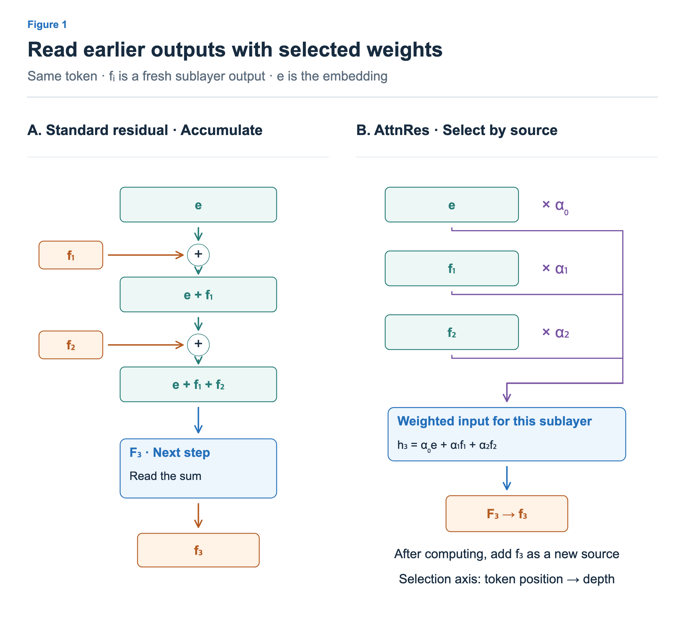
The right side weights e, $f_1$, and $f_2$ separately to form input $h_3$. Processing that input with $F_3$ produces a fresh output $f_3$. Only subsequent computations can use $f_3$ as a source. There is no cycle that reads an output before it has been computed.

Here, $f_2$ is the fresh output of the second F, not an accumulated representation such as e + $f_1$ + $f_2$. Incorrectly using accumulated representations as sources would repeat earlier contributions in multiple terms and produce a different operation from the diagram. Each fresh output can be computed from earlier results while still being stored as a fresh output.

The original AttnRes paper also motivates the design with the dilution of individual layers’ contributions as accumulated representations grow with depth in PreNorm architectures. Reading earlier results separately and assigning weights again gives control over which results contribute strongly to the current input. This describes the design objective, not a guarantee of the same benefit in every model.

The selection axis also differs from ordinary self-attention. Self-attention reads information from multiple token positions. This diagram reads already computed outputs at multiple depths for the same token position. AttnRes does not replace token mixing inside an attention sublayer. It changes the residual connection that forms the input to attention or an MLP.

Different weights produce different inputs

Suppose one token has stored e = [2, 0, 0], $f_1$ = [0, 4, 0], and $f_2$ = [0, 0, 6]. Each source is a three-dimensional vector. We give each a different nonzero component to make the arithmetic easy to distinguish. This is an educational example, not a required form for actual outputs.

Let the next layer read e, $f_1$, and $f_2$ with weights 0.25, 0.5, and 0.25. We will derive those weights in the next section. First, consider the input they produce.

Each weight multiplies an entire source vector.

Source	Weight	Contribution to the current input
e = [2, 0, 0]	0.25	[0.5, 0, 0]
$f_1$ = [0, 4, 0]	0.5	[0, 2, 0]
$f_2$ = [0, 0, 6]	0.25	[0, 0, 1.5]

Adding these three vectors componentwise gives $h_3$ = [0.5, 2, 1.5]. The weight list [0.25, 0.5, 0.25] and result vector [0.5, 2, 1.5] are different objects. The former indexes three sources; the latter indexes three feature components. The source count and vector dimension are both three only by choice in this example.

Changing the weights to [0.5, 0.25, 0.25] produces [1, 1, 1.5]. The stored vectors stay the same, but the input received by the next F changes. Selection is therefore not limited to choosing a single source. It is a continuous weighted combination that can adjust the contributions of several results differently.

A simple sum in a standard residual connection would give [2, 4, 6] in this example. Even equal AttnRes weights produce an average because softmax weights sum to one. Making the weights uniform is not the same operation as returning to the standard residual sum.

Computing weights with a learned query

We can now construct the earlier weights [0.25, 0.5, 0.25]. Each destination sublayer has a learned d-dimensional vector w, called a pseudo-query in the paper. Here, w is a learned parameter of the destination layer, not a vector obtained by projecting the current hidden state into a query.

Figure 3 separates the path that computes scores from the path that mixes originals using the resulting weights. Sources are normalized with RMSNorm for scoring. The weighted sum uses their original values before normalization.

With gain one and ε omitted, the RMS of e = [2, 0, 0] is 2/√3. Dividing gives [√3, 0, 0]. The same calculation maps $f_1$ and $f_2$ to [0, √3, 0] and [0, 0, √3]. Normalization reduces the direct effect of the original magnitudes 2, 4, and 6 on the scores.

Choose w = [0, ln2/√3, 0]. Dotting w with each normalized source gives a score of zero for e, ln2 for $f_1$, and zero for $f_2$. Here, ln denotes the natural logarithm.

Softmax exponentiates each score and divides by the sum of those exponentials. Since exp(0) = 1 and exp(ln2) = 2, the arithmetic is simple:

$$[0,\ln 2,0]\to [1,2,1]\to [\frac{1}{4},\frac{2}{4},\frac{1}{4}]$$

The resulting weights are the previous section’s [0.25, 0.5, 0.25]. Applying them to the originals [2, 0, 0], [0, 4, 0], and [0, 0, 6] gives the same input [0.5, 2, 1.5]. The √3 used in scoring is not multiplied into the originals again.

If w is a layer parameter, does every input receive the same weights? No: the sources dotted with w can change with the token and input. Even when tokens share the same destination layer’s w, different source directions can produce different scores and softmax weights. Normalization does mean that a change only in original magnitude is not passed directly into the scores.

This is a direct calculation of the report’s Full AttnRes definition in Equations (8)–(9) using the numbers above. The values of w and the sources were constructed for teaching, not extracted from a trained model.

Grouping outputs into blocks

Reading earlier outputs separately requires keeping them alive until they are needed. Retaining only the current sum, as with a standard residual connection, does not allow $f_1$ and $f_2$ to be selected separately later. Full AttnRes pays for its selection flexibility with source storage and repeated reads.

Block AttnRes sums the outputs of several sublayers along depth and stores the sum as one source. Figure 4 compares the two forms at the same instant, after $f_3$ has been computed. A block here groups sublayers along depth, not token positions in the context.

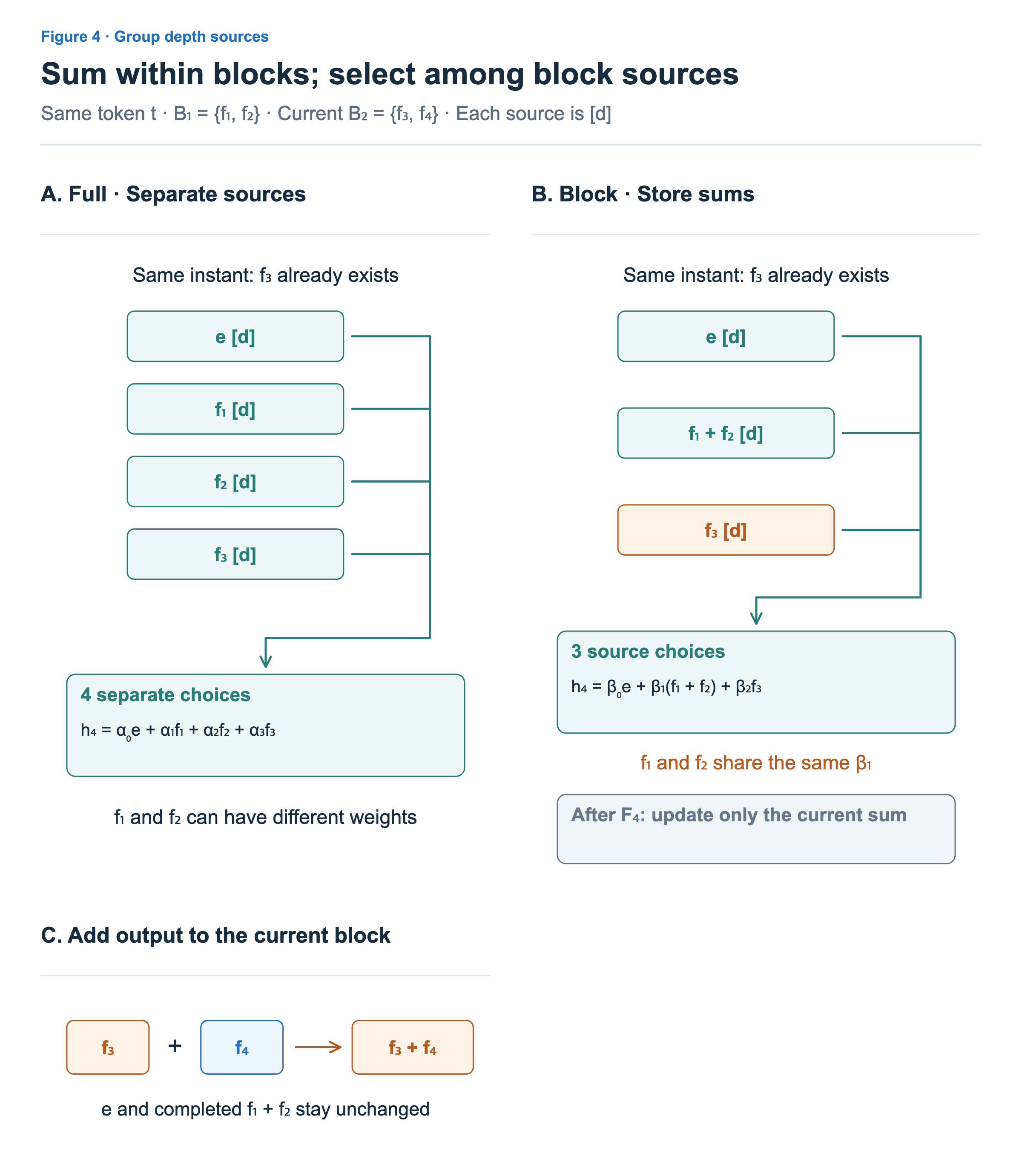
Full stores four sources: e, $f_1$, $f_2$, and $f_3$. The example Block form stores three: e, $f_1$ + $f_2$, and $f_3$. The first block is complete, while the second currently contains only $f_3$. Every source has width d.

The number of stored vectors drops from four to three, but the selection unit changes too. Full can give $f_1$ and $f_2$ different weights. Block has already added them together, so it multiplies their sum by a single weight ${\beta }_1$.

$${\beta }_1(f_1+f_2)={\beta }_1{f}_1+{\beta }_1{f}_2$$

Both share that weight. Moreover, the score is computed from the combined source rather than individual outputs, so it is not equivalent to simply adding the weights from Full. Block is not an identity transformation that produces Full’s exact result with less storage. It reduces storage by making selection coarser, at the group level.

The three current sources are read to form $h_4$, then $F_4$ computes $f_4$. Only afterward is the current block sum updated to $f_3$ + $f_4$. The embedding e and completed sum $f_1$ + $f_2$ remain unchanged. $f_4$ is not part of the read that produces itself. Under this definition, a block’s first sublayer also excludes the current sum while it is still empty.

The storage cost of depth selection

Keeping L fresh outputs separately for one token requires source storage roughly proportional to Ld. Grouping them into N block sums changes that to storage proportional to Nd. We omit small additional terms associated with the embedding and current partial sum. This comparison concerns residual source storage, not an equal proportional reduction in total training memory.

If every layer in Full reads all earlier sources, the read work also accumulates across depth. The source count grows as 1, 2, 3, …, so a straightforward calculation gives a total proportional to the square of L. Actual cost also depends on d, token count, memory access, and parallelization. The original AttnRes paper likewise distinguishes the Full structure from the Block structure intended to reduce its cost.

This source list should not be confused with a token KV cache. The separately retained values here are outputs at different depths for the same token. They serve a different role from storing keys and values at earlier positions for attention across tokens. When pipeline parallelism splits depth across devices, the cost of passing required sources to the next stage must also be considered.

The four-versus-three comparison in the diagram concerns one small example at one instant. It does not establish a 25% runtime reduction or preserved quality for a particular model. Larger blocks reduce the source count, but they also group more outputs that can no longer be selected individually.

Connecting the three residual designs

The shared question across these three articles was how information is stored between layers and supplied to the next computation. Figure 5 compares the designs using the same three criteria: storage, reading, and updating.

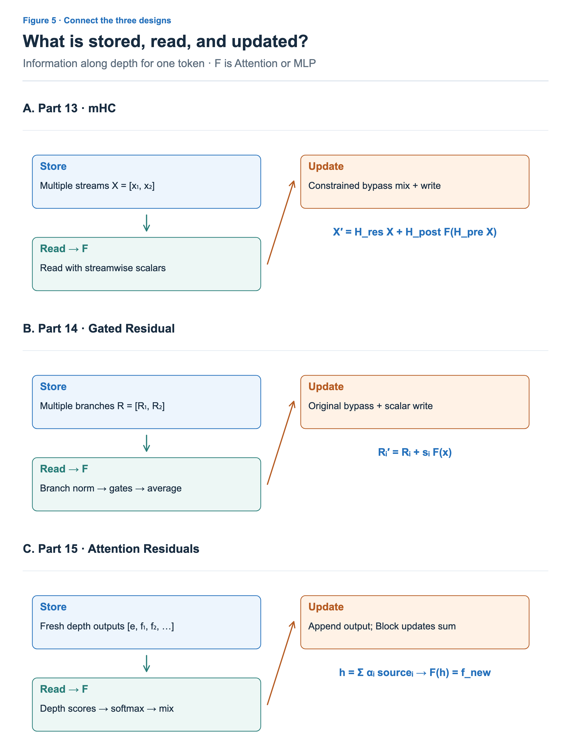
Design	Stored unit	Read for the next computation	How fresh results are incorporated
HC/mHC	Multiple concurrent streams	Combine with streamwise scalars	Add streamwise write contributions to mixed bypasses
This GR	Multiple concurrent branches	Branch norm and component gates, then average	Add a scalar multiple of the fresh output to each original
Full AttnRes	Individual fresh sublayer outputs	Depth scores and a softmax weighted sum	Append the fresh output to the source list
Block AttnRes	Depth block sums and a current partial sum	Weighted sum of block sources	Add the fresh output to the current block sum

The streams in HC/mHC and GR are not dedicated slots that preserve one specific earlier layer’s output unchanged. They are representations that are repeatedly read and updated. Full AttnRes, by contrast, distinguishes sources by the depth that produced each fresh output. Grouping both approaches together as merely “storing several vectors” misses the difference in what the next layer can select.

These variants are not mandatory replacements prompted by a failure of standard residual connections in every model. They explore richer connections, controlled reads and writes, or more direct selection of earlier results. Along with representational flexibility, they change storage and read costs, numerical stability, and implementation demands. When reading an architecture, first ask what is stored, what the next computation reads, and which values are updated. Those questions distinguish the three families more clearly than their names alone.