Cross-Layer KV Sharing: Reusing Keys and Values from Earlier Layers

MQA and GQA let multiple Query heads within a layer read the same Keys and Values. This reduces the KV stored per token, but each layer still produces its own KV.

Now we will extend sharing across layers. If the next layer also reads the Keys and Values produced by an earlier layer, the model no longer needs a separate KV bank for every layer. Cross-Layer Attention (CLA) incorporates this sharing into the model architecture. Each layer forms its own Query, while only some layers produce Keys and Values.

We will first count how storage changes across six layers, then follow one new token through two layers. Next, we will examine the computations that remain and the trade-off in extending sharing from two layers to three.

Sharing KV previously stored per layer

Each layer’s attention compares the current Query with Keys at past and current positions, then uses the resulting weights to read Values. In the basic architecture, each layer produces Keys and Values from its own input, so the same token position has different KV at different layers.

Figure 1 compares six layers after processing four tokens. Both architectures have one KV head, with two components in each Key and Value vector. On the right, adjacent layers form pairs. L₁ and L₂ read the KV produced by L₁; L₃ and L₄ read L₃’s KV; L₅ and L₆ read L₅’s KV.

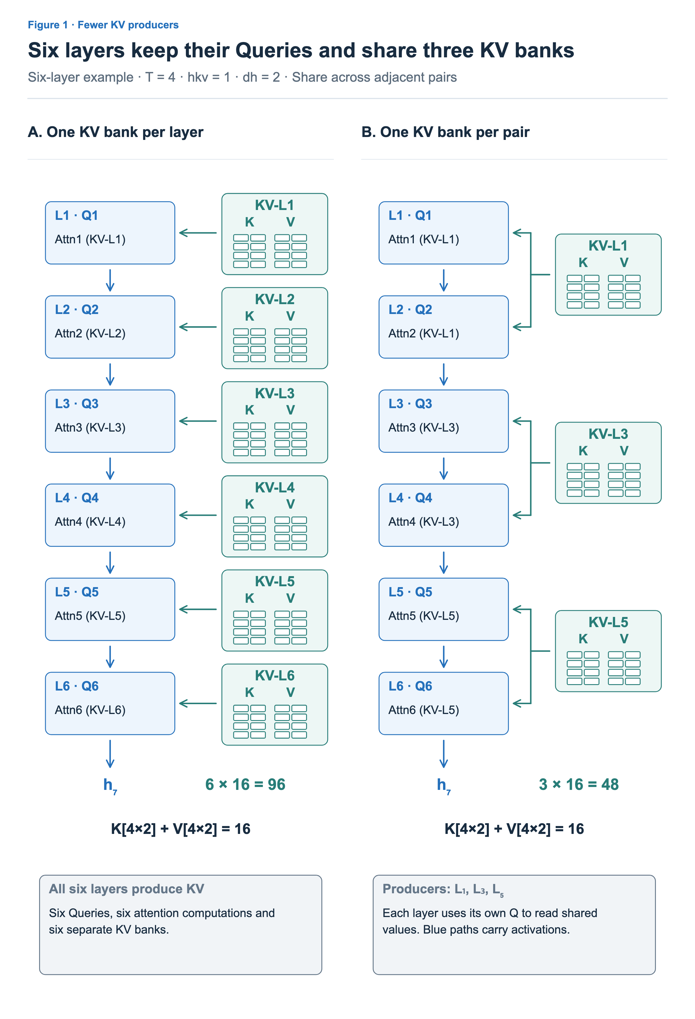
Each bank holds K[4×2] and V[4×2]. Eight Key components plus eight Value components give 16 components. Separate storage for all six layers requires 6 × 16 = 96 components, while sharing across pairs requires 3 × 16 = 48. With the same data type and tightly packed storage, this example halves the KV data size.

What decreases on the right is the number of layers producing and storing distinct KV. All six layers still perform their computations. Representations change sequentially along the blue path, and L₂ forms its Query from the representation that has passed through L₁. Even with the same KV, different Queries can produce different attention weights and outputs.

The shared objects are already computed Key and Value values. This differs from giving two layers the same KV projection weights and running each projection separately. Even identical weights can produce different KV when their inputs differ. The architecture in CLA §2.2 directly reuses KV produced by selected layers in other layers.

MQA/GQA and CLA share along different axes. MQA/GQA reduce the number of KV heads read by Query heads within a layer, while CLA reduces the number of layers producing separate KV across depth. The two approaches can be combined. We keep one KV head throughout this article to separate the effect of head count from that of cross-layer sharing.

Producing and reusing the current token’s KV

Consider only the first pair in Figure 1. KV for positions p0 through p3 is already stored, and we are processing position p4. From this position’s input $h_1$, L₁ produces Query $q_1$, Key $k_4$, and Value $v_4$. In this figure, the subscripts on q and h identify the layer; the numerals on k and v identify the token position.

In Figure 2, the orange write happens first, then the two layers read the same KV in sequence. The T=4 and T=5 boxes on the right show one KV-L1 bank before and after an update, rather than two separate stores.

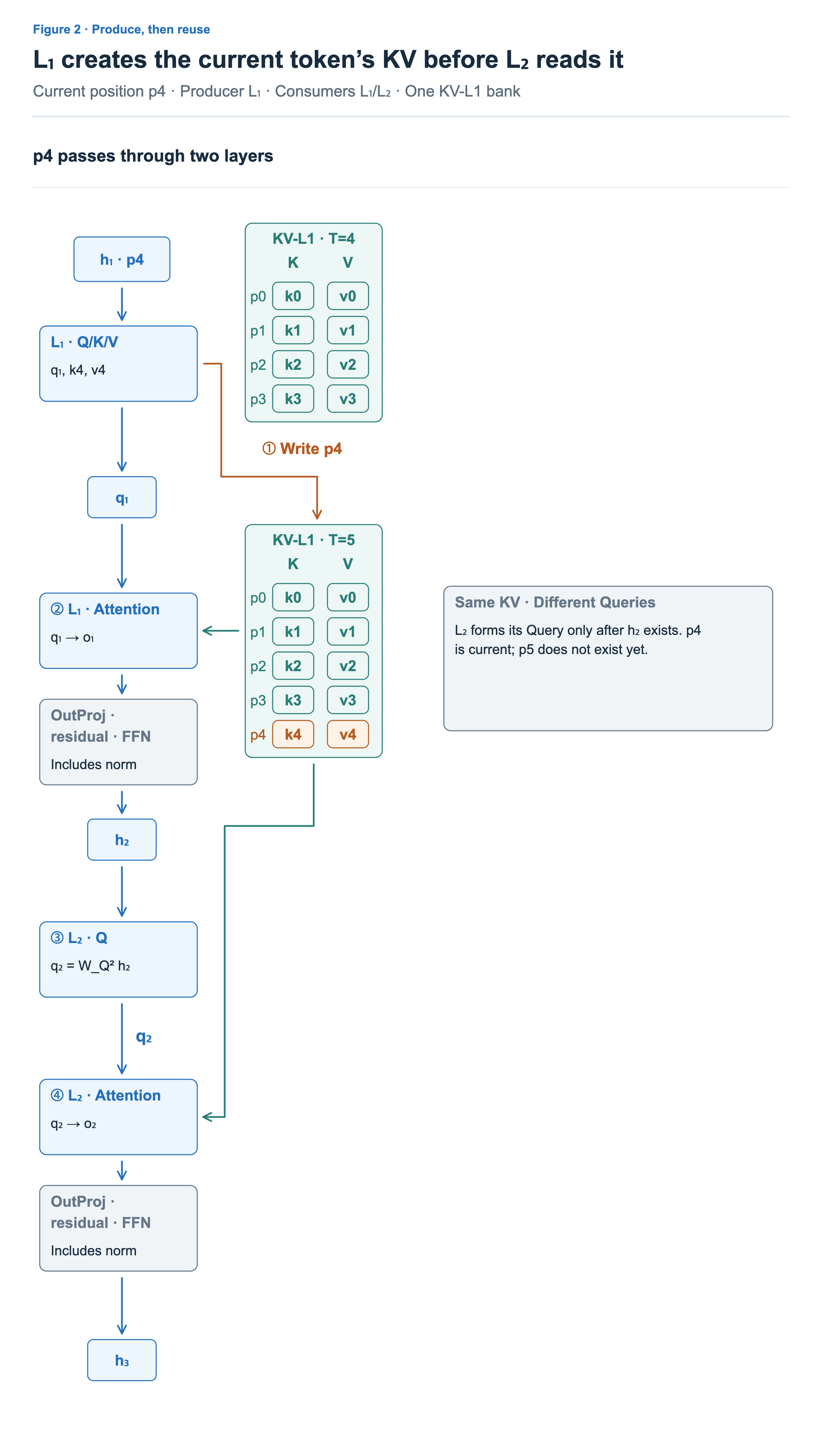
First, $k_4$ and $v_4$ are appended as row p4. KV-L1 now contains five rows, p0 through p4. Labels such as k0 and v0 name vectors at those positions, rather than their component values. Each Key and Value is two-dimensional, as in the previous section.

L₁’s $q_1$ is compared with these five Keys to obtain attention weights, which form a weighted sum of the corresponding Values. Output projection, residual connections, FFN, and related operations then produce $h_2$, the input to L₂. In the figure, o₁ is the attention weighted sum, and the gray box groups the operations that produce the next layer’s input. Normalization is included in the relevant stages; normalization before Q/K/V formation is folded into the projection box.

L₂ forms its own $q_2$ from $h_2$, then reads the five rows of KV-L1 updated by L₁. L₂ does not produce new Keys and Values from its own input or write a second p4 row into this bank. For the next token, L₁ again appends a row and L₂ reuses it.

Both layers read through the current position p4.

Reduced storage and remaining computation

Sharing KV reduces storage, but does not combine the computations through which each layer reads information. In Figure 3, count the teal stores separately from the blue computation boxes.

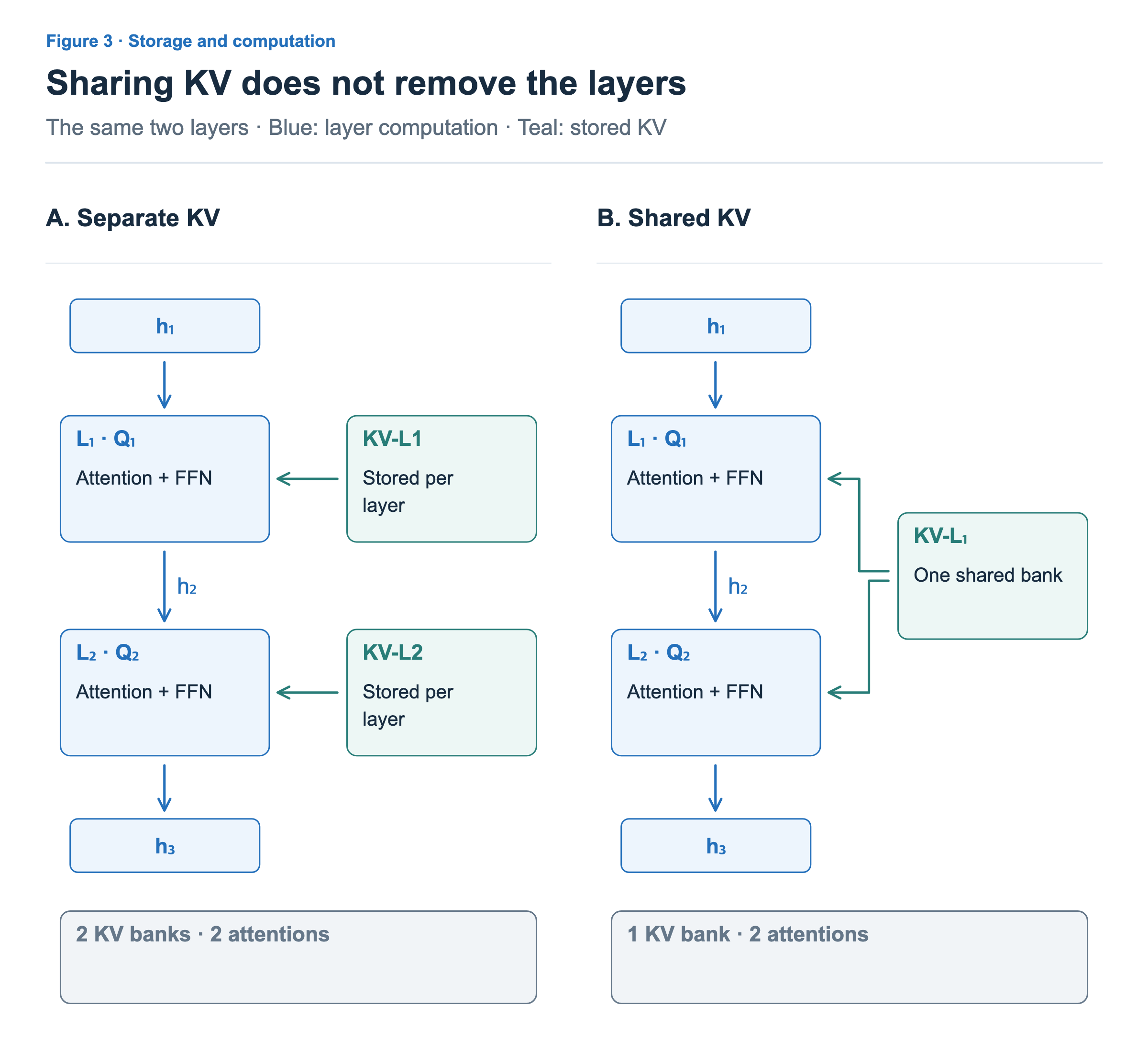
Both sides perform attention twice. The two Queries on the right score the same Key list, but the Queries differ, so each needs its own scores and weighted sum. FFN computation and sequential processing between layers also remain.

A consuming layer that does not produce its own KV can omit its K/V projections and cache writes. Those projection weights are also unnecessary. However, attention still reads the shared KV again in each layer. CLA §2.3 also distinguishes reduced KV storage from reductions in total computation and latency.

From sharing across two layers to three

The two-layer sharing used so far is CLA2. Figure 2 of the paper also compares CLA3, which groups three layers. Figure 4 keeps the same six layers and four tokens, changing only the sharing range.

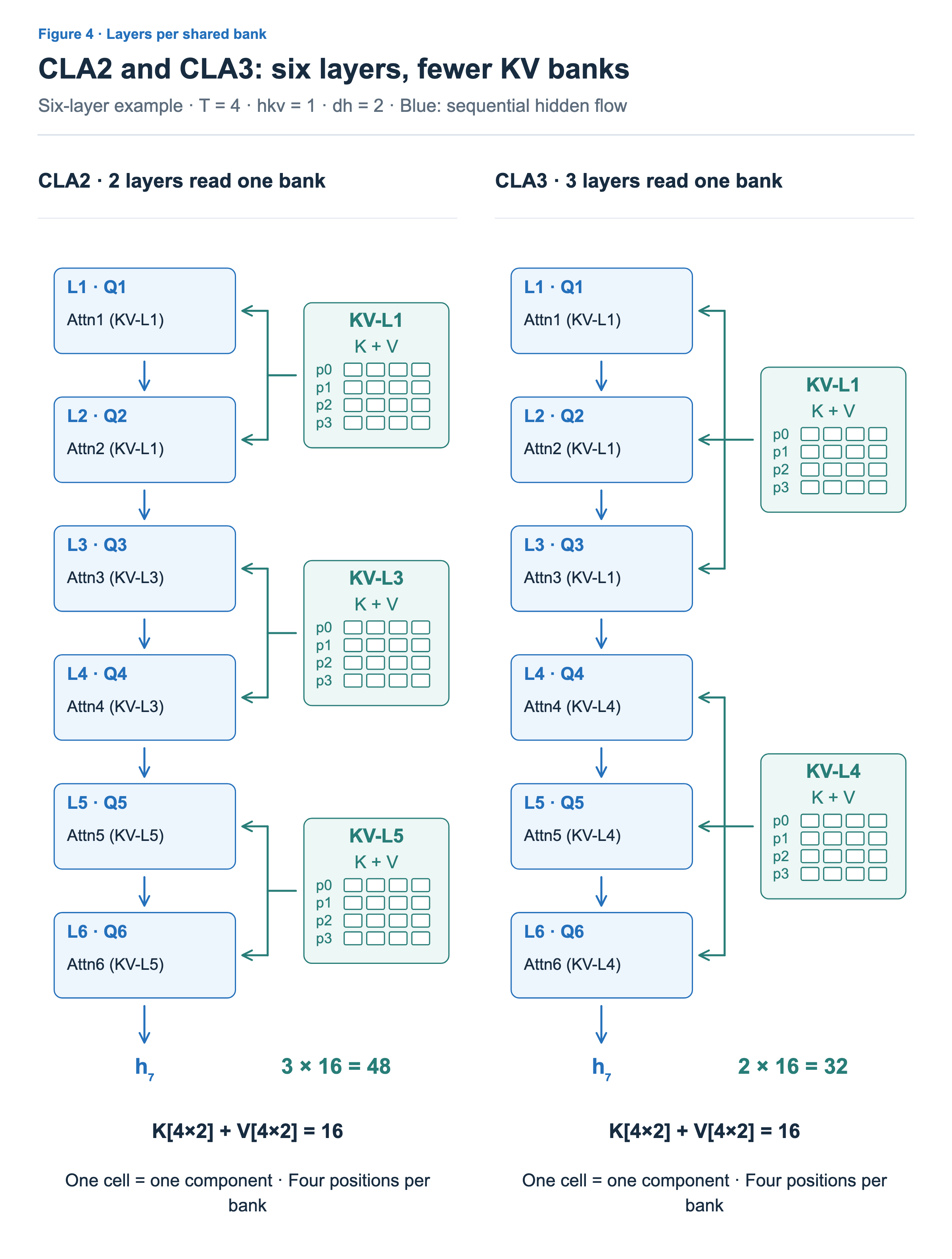
In CLA2, L₁, L₃, and L₅ produce KV, storing 3 × 16 = 48 components. In CLA3, only L₁ and L₄ are producers, so storage is 2 × 16 = 32 components. For example, L₃ produces its own KV in CLA2, but reads L₁’s KV with its own Q₃ in CLA3. Both architectures retain Query and attention computation in all six layers.

Here, 2 and 3 count the layers that read the same KV. They are not sequence compression ratios that merge three tokens into one. Every bank still stores Keys and Values for four positions, p0 through p3.

Changing the architecture has a cost. With per-layer KV, L₂ can form separate Keys and Values from its own, deeper input representation. A sharing L₂ gives up this choice and uses its own Query to read representations produced by L₁. Having different Queries does not guarantee that the two architectures produce the same output. As sharing expands, model quality must be considered alongside storage.

Cross-layer sharing is a model design that requires training for this architecture.

We can now distinguish which layers produce KV, which layers read it, and when a new token is appended. The next article examines YOCO, which separates these roles so that several later layers read KV produced by the earlier part of the model.