Learning from a Teacher’s Probabilities: OPD

In the previous article, we looked at two ways to compute advantages from task rewards: comparing responses to the same question, or comparing against a critic’s prediction of future rewards. This time, we will expand the sources of learning signals. If we have a more capable teacher model, we can read how much the teacher favors each token the student selected.

On-policy distillation (OPD) learns from a teacher’s probabilities along paths generated by the student itself. First, we will examine why we use the student’s path, then calculate the difference between teacher and student probabilities with small numbers. Next, we will distinguish forward and reverse KL by whose probabilities weight those differences. Finally, we will connect how Miles v0.1.0 adds this signal to task advantages with the case of learning from the teacher alone, without a task signal.

Learning in Contexts the Student Actually Generates

First, think of SFT, where a model learns to follow a provided answer. Suppose the training answer to a prompt P consists of three tokens: u → a → c. The student is trained to predict u from P, a from P + u, and c from P + u + a. The answer may come from a person or another model.

Now suppose that when the student actually generates a response, it chooses b instead of a as the second token. The context for the third choice becomes P + u + b. This differs from P + u + a, the context it saw when following only the provided answer. As generation gets longer, the contexts the student visits on its own can diverge further from those in the training answers.

In OPD, if the student generates u → b → d, we use that path as it is. We give the teacher the contexts the student actually passed through and have it compute the probability of the token the student selected at each point.

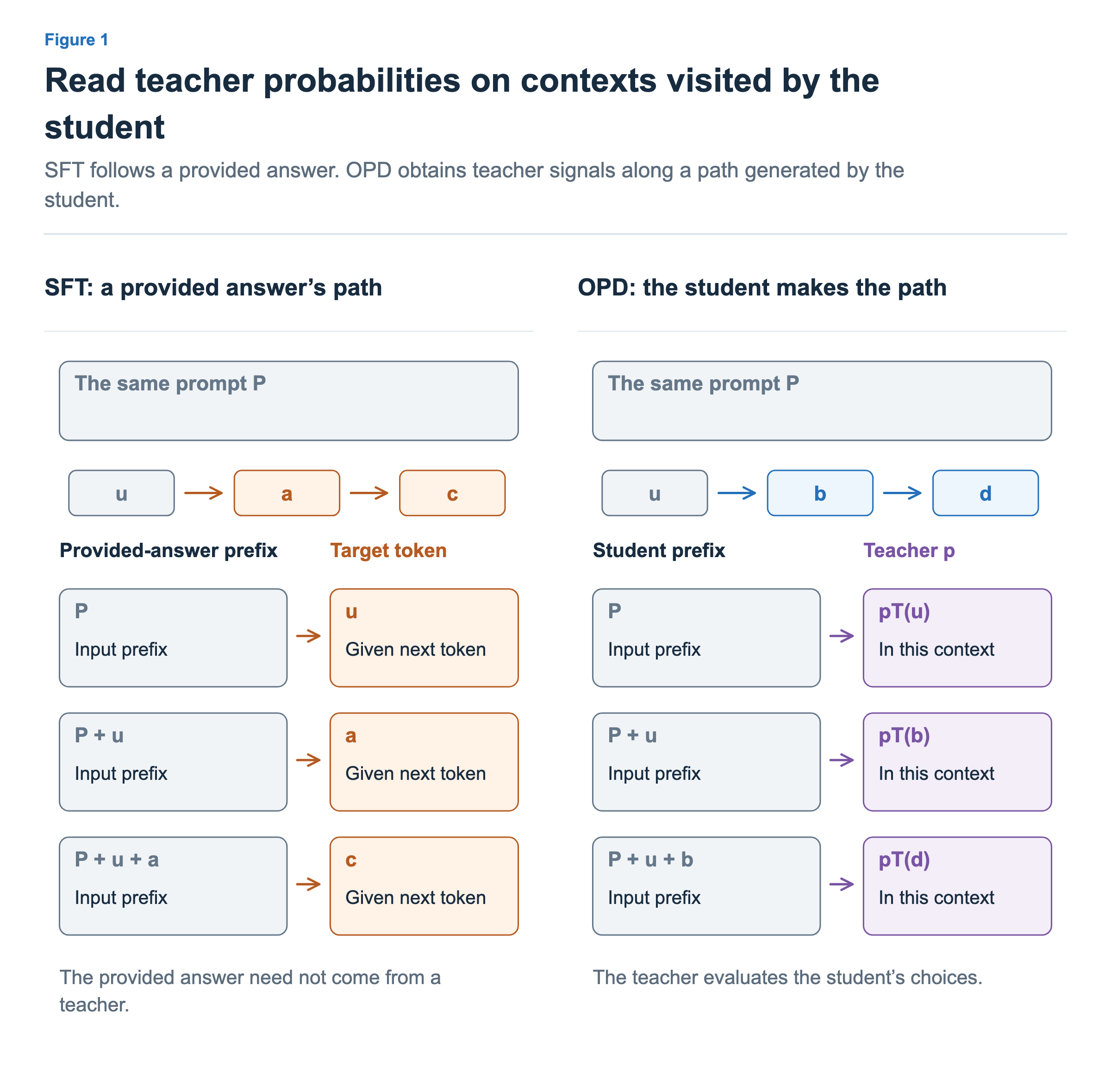
The pT(d) on the OPD path in the figure does not mean “how often the teacher uses d when writing its own answer.” It is the probability the teacher assigns to d given the student’s context P + u + b. Mistakes or detours the student commonly makes also become inputs for obtaining teacher signals. This is what distinguishes it from learning only along the path of a provided answer. Thinking Machines — On-Policy Distillation

The connecting lines in the figure show the evaluation relationship for each context. They do not mean that we must communicate with the teacher server once for every token generated. We can collect the student’s generated token history, feed it into the teacher, and obtain the log-probabilities at all positions together in a forward pass.

Comparing Probabilities for the Selected Token

Follow the second token b in the response u → b → d. Both models receive P + u. The student assigns b probability 0.2 and the teacher assigns it 0.4. Each model computes its own hidden representation, LM-head scores and softmax distribution. We then gather the probability for the same token ID b from both outputs.

In this article, we will compare the log-probabilities of a single selected token. The student probability is held fixed before this update to construct the learning signal. We compute the token-level signal dₜ as follows. ln is the natural logarithm.

dₜ = ln(teacher probability / fixed student probability)

b at P+u:   teacher 0.4, student 0.2 → d₂ ≈ +0.693
d at P+u+b: teacher 0.2, student 0.4 → d₃ ≈ −0.693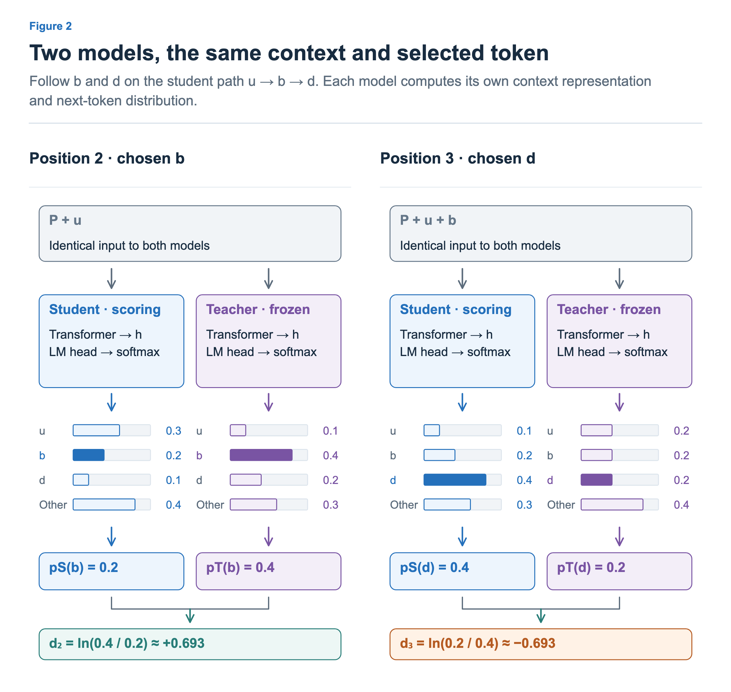

The next position has context P + u + b and chosen token d. Its student and teacher probabilities are 0.4 and 0.2, so ln(0.2 / 0.4) ≈ −0.693. The symbol dₜ denotes the distillation signal; the literal token d is an illustrative vocabulary item. The teacher sees the student’s preceding tokens, not its own independently generated answer.

If we use this value like the advantage in article 2, +0.693 acts in the direction of increasing the selection probability, while −0.693 acts in the direction of decreasing it. The sign depends on whether the teacher assigns a higher or lower probability to the student’s choice.

Here, we must distinguish the teacher’s preference from correctness on the actual task. The teacher can be wrong, and when given an incorrect preceding context, it may assign a high probability to a token that naturally continues that context. dₜ is a learning signal derived from the difference between two models’ probabilities, not a judgment of the token’s true contribution or correctness.

Which Distribution Sets the Weighting?

So far, we have compared the probabilities of one selected token. Now let us expand the view to all possible next tokens in the same context. KL divergence summarizes the difference between two probability distributions as one number. Its value depends on whether we average the differences using the teacher’s probabilities or the student’s.

For this separate example, suppose that the only candidates in context P + v are a, b and c. The teacher assigns probabilities of 49%, 49% and 2%; the student assigns 78%, 2% and 20%. Both models receive the same context, and the left and right panels use the same two distributions.

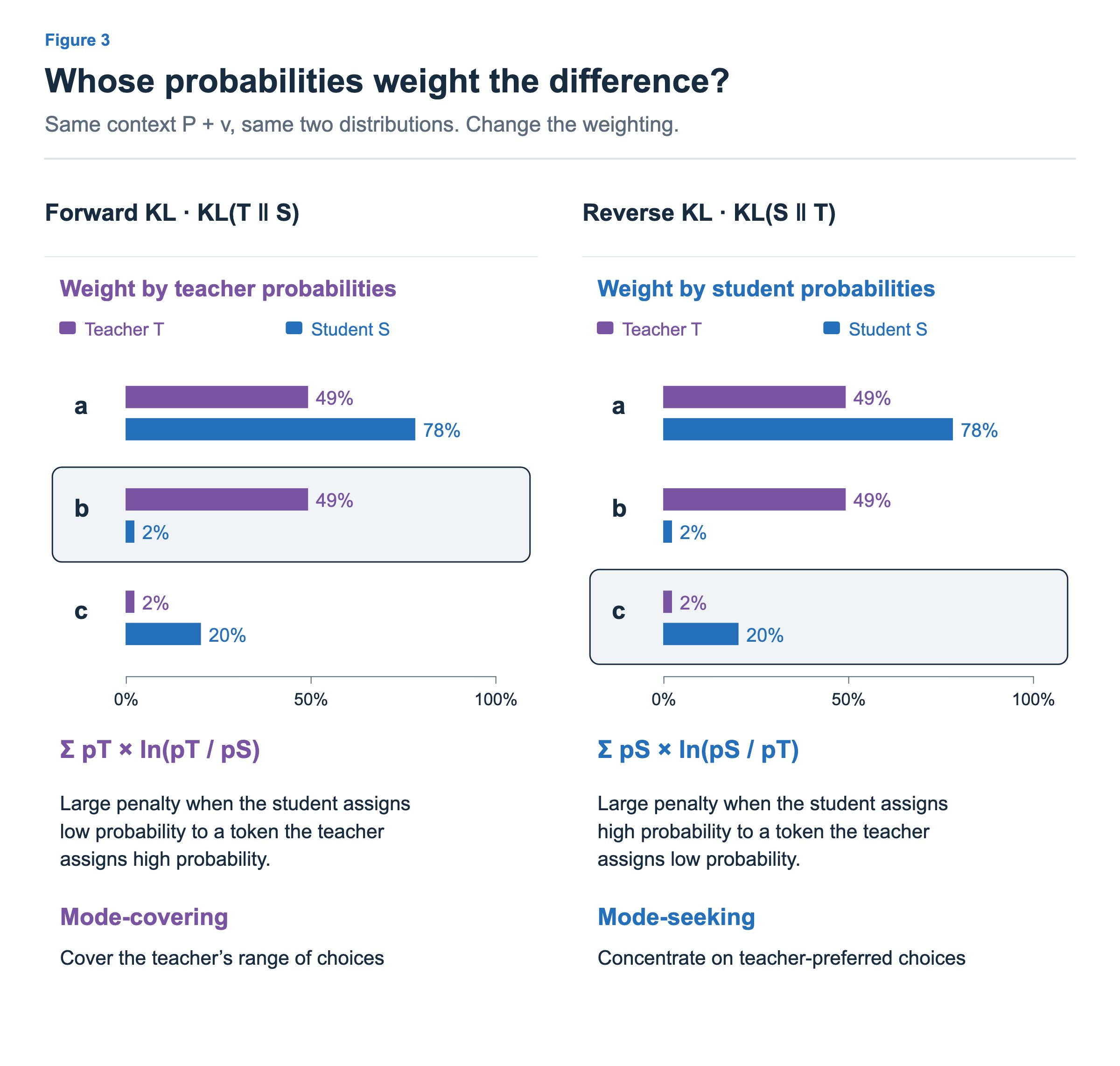
Forward KL weights by the teacher’s probabilities. Differences for tokens the teacher often selects receive greater weight. In the figure, b has teacher probability 49% but student probability only 2%. The student is almost missing one of the teacher’s choices. Writing teacher probabilities as $p_{\mathrm{T}}$ and student probabilities as $p_{\mathrm{S}}$ gives the following calculation. The shared context is omitted from the notation, and x is a next-token candidate.

$$\mathrm{KL}(T\Vert S)=\sum _x{p}_{\mathrm{T}}(x)\ln \frac{p_{\mathrm{T}}(x)}{p_{\mathrm{S}}(x)}$$

The term for b is 0.49 × ln(0.49 / 0.02) ≈ 1.57. In this example, the student’s underrepresentation of b makes a large contribution.

Reverse KL weights by the student’s probabilities. It examines whether the teacher similarly favors the tokens the student often selects. The student assigns c probability 20%, while the teacher assigns only 2%. This is a choice the student may frequently produce but the teacher rarely supports.

$$\mathrm{KL}(S\Vert T)=\sum _x{p}_{\mathrm{S}}(x)\ln \frac{p_{\mathrm{S}}(x)}{p_{\mathrm{T}}(x)}$$

The term for c is 0.20 × ln(0.20 / 0.02) ≈ 0.46. Along with reversing the ratio, we change the multiplying probability from the teacher’s to the student’s. Both KLs add the terms for all of a, b and c, not just the highlighted token. Individual terms can be negative, but the exact KL summed over all candidates is nonnegative. The total forward KL in this example is about 1.29, and the reverse KL is about 0.76. Their magnitudes alone do not tell us which training method is better. KL definitions and training configurations in GKD

The OPD signal in the previous section has the opposite sign to the log-ratio in reverse KL. Each student-sampled token receives “log teacher probability − log student probability” as a signal, and training encourages or discourages that choice. Averaging this signal under the student distribution in the same context gives negative reverse KL. A signal of +0.693 for one selected token does not contradict the nonnegativity of exact KL. Thinking Machines’ reverse-KL explanation

Also, having the student generate the contexts and using reverse KL are separate choices. We can compute forward KL in student-generated contexts by obtaining teacher and student probabilities for all candidates. This article focuses on the reverse-KL approach that uses the log-ratio of the student’s selected token as a learning signal.

Does Reverse KL Necessarily Concentrate on One Answer?

A mode is a peak in a probability distribution. Suppose the teacher’s preferred behaviors form two peaks, but the student can represent only one peak. Spreading broadly across both puts student probability in the low-probability region between them. Under reverse KL, that region, which the teacher barely supports, becomes costly. Concentrating within one peak can therefore be preferable. This is the mode-seeking tendency.

Under forward KL, missing the teacher’s other peak is costly, so a mode-covering tendency can favor covering both peaks. However, this example restricts the family of distributions the student can represent. If the student can exactly represent the teacher distribution, both KLs become zero at that distribution. We therefore will not generalize that reverse KL must concentrate on a single token or answer. GKD Figure A.16, An analysis of KL in LLM distillation

Adding Task Advantages and Teacher Signals

OPD is not necessarily an alternative that must be chosen instead of a critic or GRPO. Critics and group comparisons estimate comparison signals from task rewards. OPD provides a path for adding the teacher’s distribution as a learning target, so they can be used together.

Let us look at the basic OPD path in Miles v0.1.0 that compares tokens actually selected by the student. This is called sampled-token OPD. First, we compute the task advantage $A_{\text{task}}$ using the selected method, then add the teacher signal to produce $A_{\text{total}}$.

$$A_{\text{total}}=A_{\text{task}}+\lambda d_t$$

λ is the weight of the teacher signal. It is an OPD coefficient separate from the λ used for GAE in the previous article. In the Miles configuration, it corresponds to --opd-kl-coef. We will use an illustrative value of 0.2. The numbers below are the values immediately after addition, and the example assumes that no further normalization is applied afterward. The horizontal axes in the figure show advantage values, not probabilities or training time. Both tokens start from the same task signal and move by their respective teacher terms.

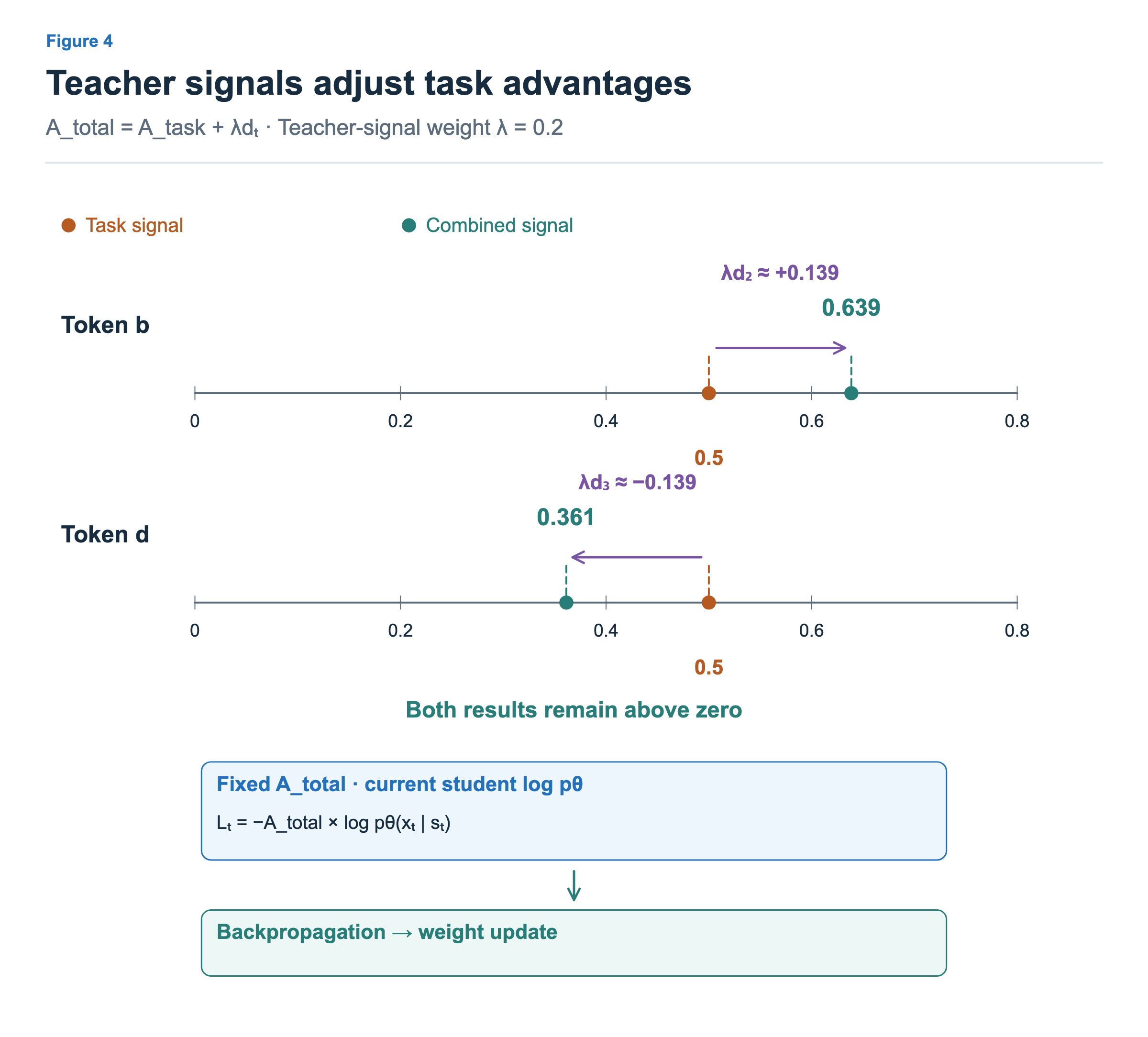
Returning to b and d in Figure 2, suppose the task provides a signal of +0.5 for both. The orange dots mark this starting point. If token b’s signal is +0.693, then 0.5 + 0.2 × 0.693 ≈ 0.639. If token d’s signal is −0.693, the result is approximately 0.361. The purple arrows show addition of the teacher terms, and the teal dots mark the combined results. The teacher signal strengthens or weakens the positive task signal.

For token d, the combined result is still positive. A negative teacher signal alone does not mean that the final policy loss will suppress that token. In this setup, we must first look at the sign and magnitude of the combined $A_{\text{total}}$. Depending on the coefficient and the magnitudes of the two signals, the final sign can also change.

For token b, the fixed coefficient is now approximately 0.639. In the basic loss, this coefficient multiplies log pθ(b | P, u). Backpropagation follows the current student’s probability computation into its LM head and earlier trainable layers. The optimizer changes student weights. It does not differentiate through $A_{\text{total}}$, the teacher, or the stored token IDs.

When GRPO and OPD are used together, a different teacher term for each token is added to GRPO’s advantage shared across a response. Miles can normalize advantages after this addition, depending on the configuration. The subsequent probability ratios, clipping, and loss aggregation follow the policy loss path of that training setup. The point of addition and the signs of the signals can be checked in the Miles v0.1.0 OPD implementation.

Why a Policy Loss Exists Without Task Scores

What happens if we set the task advantage to 0? Imagine moving the orange starting points in Figure 4 from +0.5 to 0. The teacher terms stay the same, so only $A_{\text{task}}$ disappears from the calculation above; λ × dₜ remains. The final signals for the two tokens are approximately +0.139 and −0.139.

The student’s policy loss uses these signals and the student’s current probability computation. In the basic explanatory formula, it is −A_total × log p_current; in a setup with probability ratios and clipping, $A_{\text{total}}$ enters that setup’s objective. The difference between teacher and student probabilities can therefore support learning even when the task signal is 0.

The teacher does not directly output the final loss. It provides probability information, and the training code uses that information to construct a signal before computing the specified policy loss. This is the same distinction we made in article 2, where the reward was not the loss itself.

The pure OPD example in Miles provides a path that returns 0 for task rewards. In a setup such as GRPO, where the group mean is subtracted from each task reward, the task advantage becomes 0 and the teacher term remains. However, we must not generalize that setting rewards to 0 immediately makes $A_{\text{task}}$ 0 for every advantage estimator. In setups where critic predictions or other reward or regularization terms remain, we need to inspect the actual computation path. This OPD addition changes the advantages while leaving the return targets unchanged, so the teacher signal does not automatically enter the critic’s training targets. Miles v0.1.0 rollout and reward handling

When to Compute and What to Hold Fixed

One training path proceeds in the following order.

1. The student generates a response to a question and records its context and token history.
2. The teacher’s token-level probabilities are computed from the same history.
3. They are compared with student probabilities held fixed for signal construction to produce dₜ, which is added to the task advantages.
4. The policy loss is computed using the current probabilities of the student being trained, and gradients are backpropagated to the student’s weights.

We need to distinguish the student probabilities used to construct the signal from the current student probabilities differentiated in the policy loss. Depending on the configuration, Miles uses either log-probabilities recorded during generation or log-probabilities from evaluating the student model before the update to compute the signal, then holds that signal fixed. The policy is made to change its selection probabilities according to the given signal, rather than changing the signal itself to reduce the loss. Miles v0.1.0 advantage computation

There are also choices about where to run the teacher’s computation. Miles’ SGLang teacher mode places information obtained from an external teacher server into the rollout data, while its Megatron teacher mode obtains it from a teacher forward pass on the training side. Neither mode updates the teacher’s weights through this policy loss. This token-level comparison also assumes that the student and teacher can interpret the same token IDs with the same meaning. Miles v0.1.0 OPD documentation

What Role Does the Teacher Model Play?

We can now distinguish the models with similar-sounding names by their roles.

Role	Information provided in this series
Reward model or verifier	An outcome score based on the task’s criteria
Critic	A prediction of the future return from the current context
Fixed reference	Probabilities from the comparison baseline we want to retain during training
OPD teacher	Token probabilities that serve as learning targets in contexts visited by the student

A fixed reference and a teacher can both provide probabilities, but they serve different purposes in training. The reference manages deviation from a chosen baseline, while the teacher provides a distribution of behavior for the student to learn. Which role a particular checkpoint plays is a choice in the training design.

OPD does not have to be implemented only through the advantage-addition formula in this article. Other approaches directly construct a distillation loss from the difference between distributions or use probabilities for multiple candidates beyond the selected token. Miles also has a separate signal computation using top-k candidates. This article has focused on the basic sampled-token path to explain the connection between student contexts, fixed teacher signals, and the student’s policy loss.

There need not be just one teacher. We can extend the approach by sending math problems to a math teacher and coding problems to a coding teacher. Miles’ multi-teacher routing selects one teacher per sample; it does not necessarily average the probabilities of all teachers. GLM-5 describes cross-stage OPD that uses checkpoints from earlier SFT and RL stages as teachers to recover capabilities weakened during subsequent training. GLM-5 §3.5

The next article will place RL and OPD within an overall training strategy. Starting with DeepSeek V4’s specialist training and multi-teacher integration, we will compare OPD before RL and MiMo’s extension with multiple prefixes.