RL · 2026-09-25
Computing Advantages with Groups and Critics
Start with GRPO comparisons within a prompt, examine critic predictions and advantages, then connect them to single-rollout learning in SAO and FlashREINFORCE.
In the previous article, we explained that an advantage computed from rewards provides a signal for favoring a selected token more or less. For example, a return of 1 and a baseline of 0.4 gave us a signal of +0.6. Where, then, does this baseline of 0.4 come from?
We will first compare several responses to the same question, then introduce a critic that predicts future rewards from the current context. Both supply a baseline for advantages. Finally, we will connect this choice to the experience that must be collected before learning, including approaches that use one rollout per prompt.
GRPO Compares Responses to the Same Question
A simple starting point is to use the outcomes of other generated responses as the baseline. GRPO (Group Relative Policy Optimization) generates multiple responses to the same question and compares their rewards. Here, we will consider the basic outcome-only setup, which evaluates only at the end of a response. DeepSeekMath §4.1
Suppose we generate four responses to one question and receive rewards of [1, 1, 0, 0]. These four responses form one group. Their mean is 0.5, and their population standard deviation is 0.5. We subtract the mean from each reward and divide by the standard deviation. Subtracting the mean reveals whether the outcome was better or worse than the baseline, and dividing by the standard deviation expresses that difference in units of the group scores’ spread.
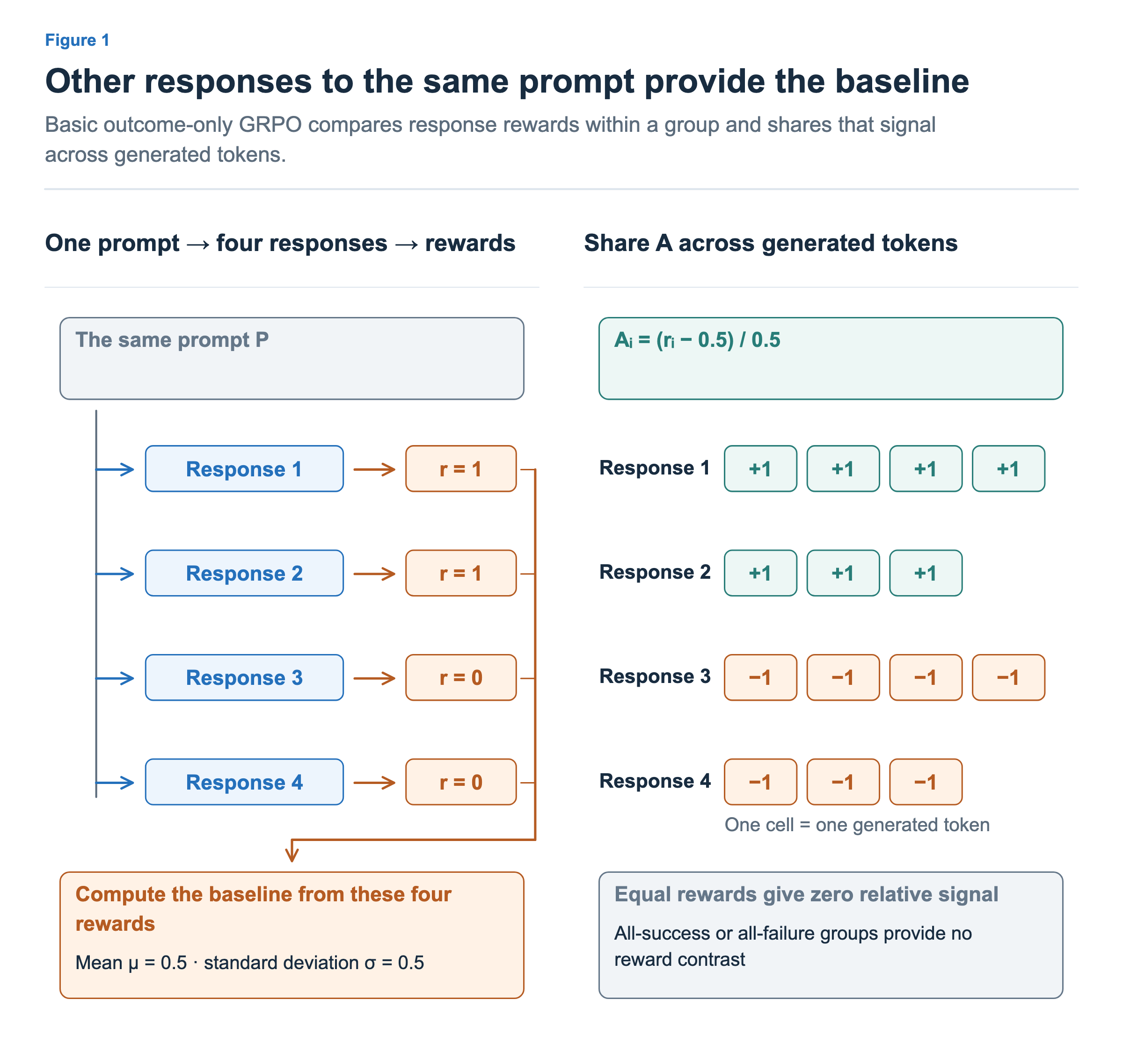
For the two successful responses, (1 − 0.5) / 0.5 = +1; for the two unsuccessful responses, (0 − 0.5) / 0.5 = −1. In this setup, the value obtained for each response is shared across that response’s generated tokens. This does not mean that the input question or text returned by tools is also treated as tokens selected by the policy.
Using the same A for all generated tokens is not a claim that every token contributed equally. It is a way of using a response’s relative evaluation in the policy loss for each choice. The current probabilities and probability ratios still differ from token to token, so the same A does not mean the same loss or the same magnitude of weight change.
Responses to other questions are not mixed into this group mean. Rather than directly comparing absolute scores across easy and difficult problems, we examine which responses were relatively better for the same question. Standard deviation calculations and normalization methods can vary by implementation, so the exact +1 and −1 above are examples under the stated calculation convention.
What if all four responses succeeded or all four failed? Subtracting the mean from each reward gives 0 in every case, so there is no relative reward difference. The standard deviation is also 0, so we cannot perform the simple division as written. With numerical handling such as adding a small ε to the denominator, this relative reward signal becomes 0, and some setups exclude such groups from training. This does not mean that separately added KL or teacher signals are also all 0.
A Critic Predicts Future Outcomes
Imagine that a model is partway through generating a mathematical answer and is looking at what it has written so far. The final answer has not appeared yet, but we can still estimate how good the outcome will be if it continues from here. Predicting that expected value is the role of the critic—in this case, a value model that predicts state values.
We write the value obtained by feeding the current context sₜ into the critic as V(sₜ). V predicts the return that will be received as the policy chooses subsequent actions from that context. If the only rewards are 1 for success and 0 for failure, with no additional weighting of future rewards, we can interpret it in terms of expected success. If the reward includes other terms, V predicts that return too, so it is not always a probability of success.
This differs from the role of the reward model we saw earlier. A reward model or verifier applies evaluation criteria to the generated result, while a critic predicts subsequent outcomes from an unfinished context. A high value from the critic does not mean that the answer has actually been verified as correct.
An LLM critic can be built by adding a layer that outputs a single number from the language model’s context representation. In this article, we will consider a critic trained separately from the policy. The critic does not generate its own complete answer and then have it scored; it computes V from the given context. Even when the entire token history is processed at once during training, each position’s prediction must be prevented from reading future tokens in advance.
The Same Final Reward, Different Predictions
Consider the illustrative response u → b → d from the previous article. The corresponding contexts are P, P + u, and P + u + b. The critic’s predictions immediately before each action are 0.2, 0.6, and 0.4, and the actual reward is 1 only at the end. These are hypothetical numbers for explanation. P denotes the input prompt. We will start with the simplest comparison between a fully observed outcome and the prediction at each point.
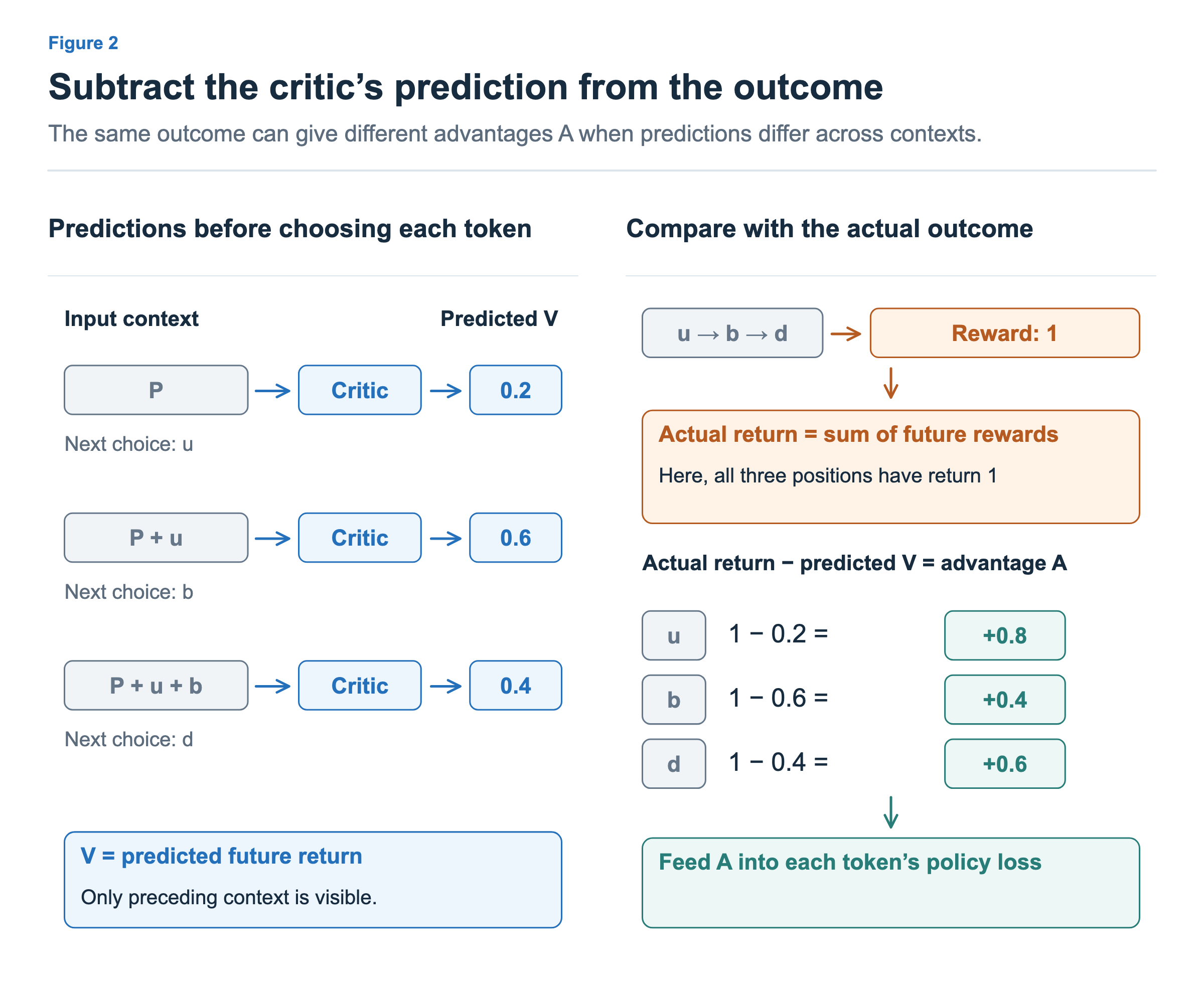
On the left, the critic predicts future rewards from the context immediately before each token is chosen. Its prediction is 0.2 with only P, 0.6 after generating u, and 0.4 after generating b. The same critic is applied at three positions; these are not three separate critics. V can rise or fall with the context. It predicts future rewards from the current context rather than accumulating past accomplishments.
On the right is the actual outcome known after completing and scoring the response. Return is the accumulated reward received from that point onward. This example uses no discounting, has zero intermediate rewards, and receives 1 only at the end. The sum of subsequent rewards is therefore 1 before every token.
Subtracting predicted V from this actual return gives advantage A, a signal of how much better the outcome was than expected. For u it is 1 − 0.2 = 0.8; for b, 1 − 0.6 = 0.4; and for d, 1 − 0.4 = 0.6. Each A enters the corresponding token’s policy loss introduced in the previous article.
Using these values as the advantages A₁, A₂, and A₃ at the respective positions produces signals of different magnitudes even within the same response. This does not mean that the first token contributed 0.8 to the correct answer. We are comparing the difference between the prediction from each context and the realized outcome.
The critic itself must also be trained. In this example, we use the subsequently observed return of 1 as the training target and reduce the error so that the prediction V from each context moves closer to that target. The simplest value loss is (V − 1)². While the policy loss adjusts token selection probabilities, the value loss adjusts the critic’s predictions of future rewards.
Thus, saying “the critic determines PPO’s advantages” is a somewhat abbreviated description. The critic provides the predictions needed for comparison. A is obtained by putting both the actual rewards and those predictions into the advantage calculation.
Going further: from one-step prediction changes to GAE
Instead of using only the return observed all the way to the end from each point, we can also use the prediction at the very next point. We compare the current prediction with the reward just received + the reward predicted to remain in the next state. This difference is called the TD (Temporal Difference) error, written δ (delta). A is the advantage used in the policy loss; δ is a one-step prediction error used to compute that A.
TD error δₜ = reward just received + γ × V of the next state − V of the current stateγ is the discount factor that determines how much to account for future rewards. Setting γ = 1, as in the example, gives the following three calculations.
δ₁ = 0 + 0.6 − 0.2 = +0.4
δ₂ = 0 + 0.4 − 0.6 = −0.2
δ₃ = 1 + 0   − 0.4 = +0.6
The final 0 means that the response has truly ended and there are no more rewards to receive. It does not mean that every temporary pause or cutoff caused by a length limit can be treated as the same kind of termination. Whether to use the value beyond that point depends on whether the state will continue.
GAE (Generalized Advantage Estimation), widely used with PPO, estimates advantages by accumulating these TD errors from subsequent points. It uses the current error as is, then weights more distant errors by γλ, then (γλ)², and so on. λ controls how far into the future the errors are taken into account. GAE paper
Setting both γ and λ to 1 here lets us simply sum the subsequent errors. A₃ is 0.6, A₂ is −0.2 + 0.6 = 0.4, and A₁ is 0.4 − 0.2 + 0.6 = 0.8. These are the same results we obtained earlier by subtracting each V from the final return. The TD error just after choosing b is −0.2, but A₂ becomes +0.4 when the later error of +0.6 is included. This distinguishes comparing against a one-step prediction from incorporating later outcomes. With λ = 0, later TD errors are not added: the current δ itself is used as an advantage estimate.
This equality holds for a fully observed response with γ = λ = 1. GAE is not always computed as “final score − V.” By adjusting how much to incorporate distant observations versus relying on the critic’s predictions at nearby points, it trades off bias and variability in the estimate. This is why the quality of the critic’s predictions also matters during training.
Changing the Baseline Changes the Work Required
One reason GRPO attracted attention is that it can compute advantages without a separate critic. It can reduce the burden of storing critic parameters and training state, computing V, and learning from prediction errors. DeepSeekMath also identifies this memory and computation burden as a major motivation. DeepSeekMath §4.1.1
In exchange, obtaining a group baseline requires generating and scoring multiple responses to the same question. PPO can also generate multiple responses, so this does not mean that every PPO and GRPO run must generate different amounts of data. The cost of a critic and the cost of group generation come from different kinds of work. Which is cheaper depends not only on model size but also on response length, group size, and resource placement.
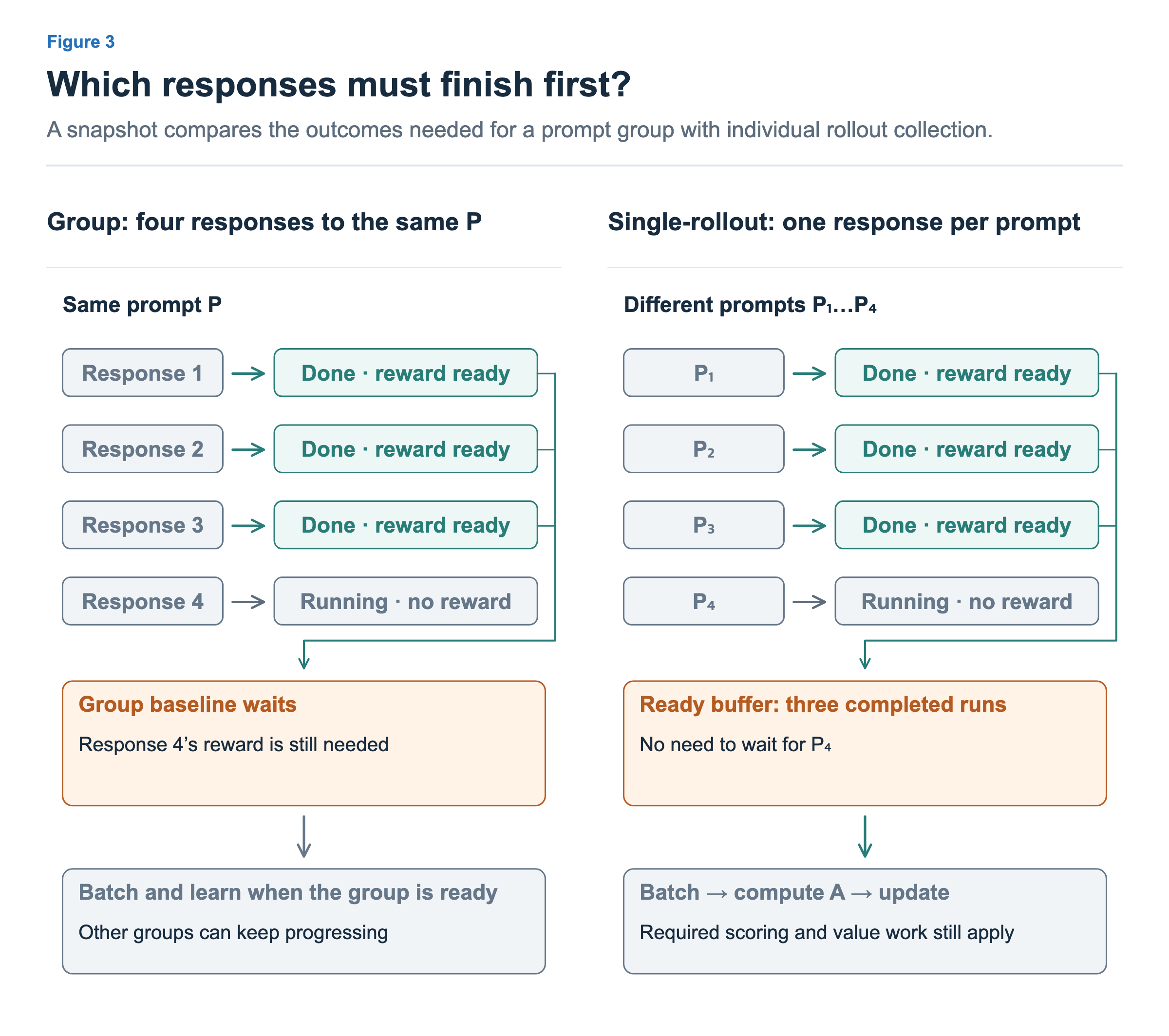
The left side shows four responses generated for the same prompt P. Three have been scored, but one is still running. Computing the mean and spread of all four rewards requires that last result too. This is not a speed measurement: it shows which outcomes the baseline depends on.
Once a response finishes, its generation slot can serve another job. When an individual job releases resources differs from when the group’s advantages are ready. Generation for other groups and training on ready data can also continue.
With long reasoning responses, some samples can produce far more tokens than others. Multi-turn agents may also execute code, read the results, and generate again. A slow tool call or more attempts can extend the completion time of a job. In such cases, it matters not only how fast generation runs, but also when each group becomes ready in the presence of slow samples.
Learning without Same-Prompt Siblings
The right side of Figure 3 generates one rollout for each of the distinct prompts P₁ through P₄. The three completed runs can enter a ready buffer while P₄ continues. There is no dependency requiring them to collect sibling responses to the same question. Three is an illustrative count, not a specified batch size. One rollout per prompt does not mean batch size one or an immediate optimizer step. Actual updates still require batching and any necessary scoring and value computation.
A baseline is still needed, and a critic is not the only option.
| Approach | Advantage baseline | Same-prompt siblings required? |
|---|---|---|
| Basic GRPO | Reward mean and spread for that prompt | Yes |
| SAO | Critic predictions combined with observed rewards | No |
| FlashREINFORCE | Reward mean of a completed batch across prompts | No |
SAO (Single-Rollout Asynchronous Optimization) retains the actor–critic structure familiar from PPO and adapts it to asynchronous agent learning. Its single-rollout design avoids waiting for sibling outcomes. It also adjusts importance correction and critic training to handle stale experience. The underlying division of labor remains: the critic predicts returns, rewards and predictions produce advantages, and the actor updates token probabilities. SAO §§3–3.2
FlashREINFORCE instead centers rewards across completed runs from different prompts, using Aᵢ = Rᵢ − batch mean. For rewards [1, 1, 0], the mean is 2/3 and the advantages are approximately [+0.33, +0.33, −0.67]. It uses a fresh completed batch for one update, then discards it. FlashREINFORCE — One-Batch REINFORCE
Figure 4 compares only the paths for computing A from the same completed experience. The rewards for three distinct prompts are 1, 1 and 0.
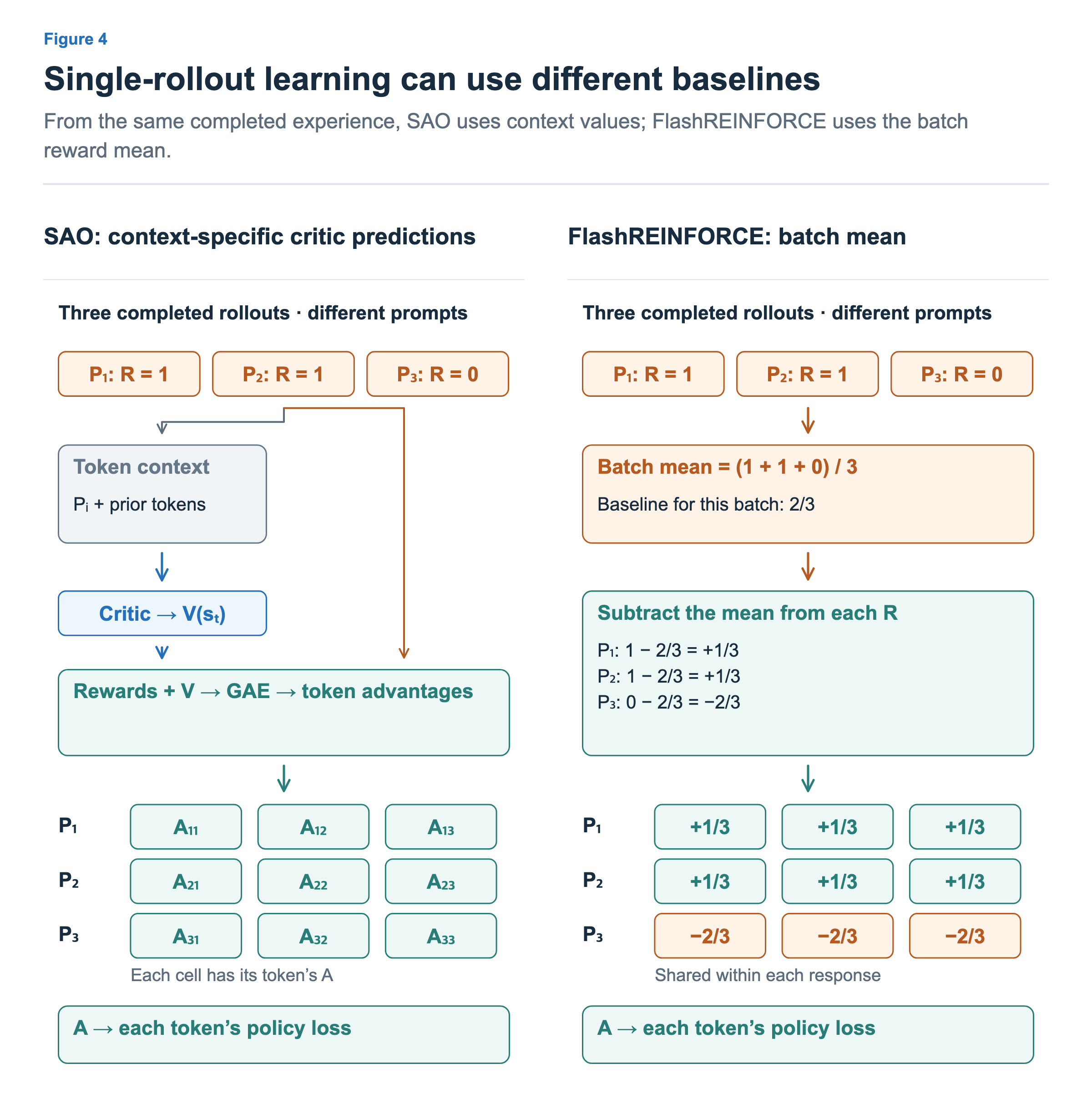
On the left, each rollout’s contexts enter the critic to produce V, which is combined with actual rewards through GAE to obtain A. A₁₁ is the advantage of the first generated token in the first rollout; A₁₂ belongs to its next generated token. Values can differ within a response. SAO also adjusts GAE so that observation tokens returned by tools are not treated as policy actions. SAO §3.2
On the right, the mean reward of 2/3 is subtracted without a critic. The first and second responses receive +1/3, and the third receives −2/3; each value is shared across that response’s generated tokens. Unlike GRPO in Figure 1, the baseline comes from a completed batch across distinct prompts. The three cells represent generated tokens and do not imply that all responses have equal length.
Both paths feed A into policy losses. This figure focuses on the baseline; it does not imply that the algorithms use identical importance correction or masking.
That cross-prompt mean is not a prediction of how difficult each particular problem is. It trades precise same-prompt comparison for broader prompt coverage and simpler collection. A successful easy problem and a failed hard problem do not become equally informative just because their rewards share a baseline. This is a different estimator and data-collection choice, not proof that a critic is unnecessary in every setting.
Long tasks also change the unit of experience. GLM-5.2 reports that context compaction splits one task rollout into trainable sub-traces whose counts and lengths differ across runs of the same prompt. It uses critic-based PPO to train on individual rollouts and includes all compacted sub-traces with token-level loss. GLM-5.2 — Long-Horizon RL
For intuition, one run might yield two sub-traces while another yields five. These are segments of two original attempts, not seven independent answers. This example is illustrative. Variable length does not make GRPO mathematically impossible; it raises decisions about grouping, credit assignment and weighting. A critic is one way to obtain context-specific predictions without constructing a sibling comparison for every segment.
Historically, PPO preceded GRPO, and removing the critic helped make GRPO attractive. Recent single-rollout work does not establish a universal progression back to critics. Whether to learn a value model and whether to require a same-prompt group are separate choices. Their usefulness depends on the task, experience structure and collection cost.
Where Time Goes in Runs with Long Generation
The process of generating responses to obtain experience for learning is called a rollout. Let us look at one public measurement to see whether generation can actually account for a large share of time. The Skywork-OR1 report gives the following times for a 32B model run over 1,000 steps. Policy update refers to the update phase that includes the current model’s probability computation and backpropagation, or its forward and backward passes. Skywork-OR1 §5.1, Table 7
| Phase | Reported time | Approx. share of the 309-hour total |
|---|---|---|
| Rollout | 223 hours | About 72% |
| Policy update | 27 hours | About 9% |
| Other | 59 hours | About 19% |
Dividing the reported times gives a rollout duration approximately 8.3 times that of policy updates. In this run, reducing generation time has the potential to affect total elapsed time more than speeding up update computation alone.
These are results from the run in that report. They do not represent the time proportions of all LLM RL runs, and we should not attach a GPU configuration from a separate experiment to this table and generalize from it. When generation and training overlap asynchronously, we also cannot obtain the total time by simply adding the times of the individual phases. We will carry this distinction forward into the later articles on systems and measurement.
In the next article, we will look at another path for obtaining a comparison signal: on-policy distillation, which reads a teacher model’s token probabilities in contexts actually generated by the student and uses the difference as a learning signal.