How Rewards Change Token Generation Probabilities

In the previous article, we followed how an LLM chooses tokens one at a time to produce a response and receives a reward for the completed response. Now suppose a correct response has received a score of +1. This number alone does not tell us which model weights to change or in which direction. We need to connect the evaluation result to the model’s computation.

First, we recompute the current probabilities of the recorded tokens and use the reward to calculate an advantage that indicates how much more we should favor this choice. After understanding the basic path that connects these two values in a loss, we will add probability ratios and clipping for training on the same data again. Finally, we will distinguish the role of a reference policy in keeping the model from moving too far from its starting point.

Recomputing the Probability of an Already Selected Token

The training data records which token was selected in which context. We will write the context at token position t as sₜ and the token selected there as xₜ. θ represents the weights of the model currently being trained.

Feeding the same context sₜ into the current model lets us compute the probabilities of the candidate next tokens. The probability we extract for the recorded token xₜ is pθ(xₜ | sₜ). The vertical bar means “given this context.” We are not generating a new response here. We are recomputing how plausible the current model considers the recorded choice.

We will write the prompt as P. Suppose the recorded response to prompt P consists of the illustrative tokens u → b → d. To score u, the model sees P; to score b, it sees P + u; to score d, it sees P + u + b. These are three prediction positions of the same model, not three separate models.

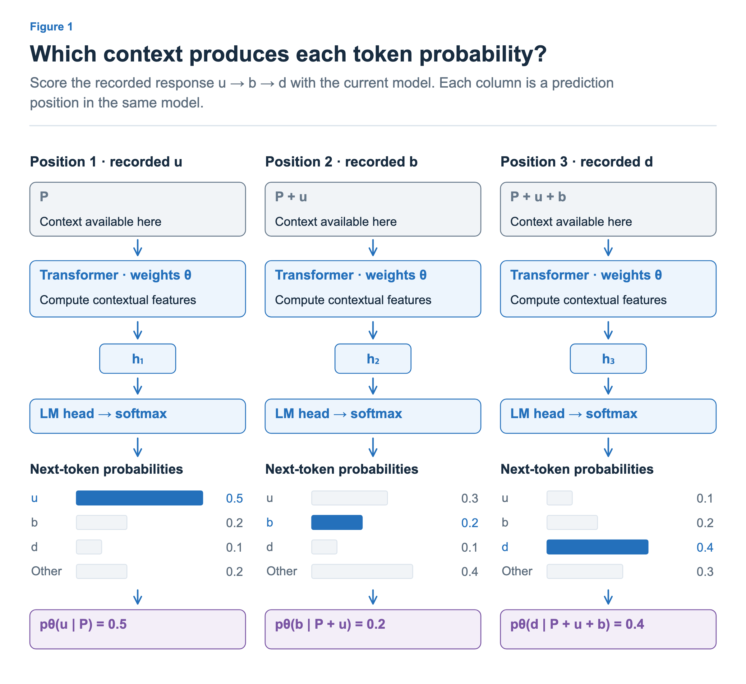
At each prediction position, the Transformer computes a context representation hₜ. The LM head maps it to a score for every vocabulary token, and softmax turns those scores into probabilities. We gather the probability of the token that was actually selected. Thus the second position uses pθ(b | P, u) = 0.2, even if another candidate has a higher probability. “Other” in the figure combines all remaining vocabulary tokens; these numbers are illustrative.

During generation, tokens must be sampled in sequence. During training, the recorded sequence is already available, so these positions can be evaluated together with a causal attention mask. The position predicting b cannot see b or the later d. The training forward pass retains the computation needed for backpropagation; it does not differentiate through the earlier sampling decision.

For example, if the selected token’s current probability is 0.5, its natural logarithm is approximately −0.693. At a probability of 0.6, the log-probability is approximately −0.511. As the probability increases, the log-probability increases too. The log-probability itself is neither correctness nor a reward. It is a result of the model’s computation whose change with respect to the weights can be differentiated.

Computing an Advantage from Rewards and a Baseline

Now let us look at the input from evaluation. The accumulated rewards received after a choice are called the return. In a simple example where a reward of +1 is received only at the end and rewards are weighted equally regardless of when they arrive, the observed return is 1 for the choices within that response.

Yet the same score of 1 can provide a different learning signal depending on whether it was easy to obtain or better than expected. We introduce a baseline for this comparison. The simplest form is:

advantage = observed return − baseline
               1          −   0.4    = +0.6

An advantage is an estimate of how much better the outcome of a choice was than the baseline. The +0.6 in this example means that the outcome was better than the baseline. If the return had been 0 with the same baseline, the advantage would be −0.4, providing a signal to favor that choice less.

The baseline can come from a critic that predicts the expected reward from the current context, or from the scores of several responses generated for the same question. The former is commonly used in PPO, while the latter is the central idea of GRPO. We will cover the detailed calculations in the next article. The key point at this stage is that rewards and advantages are different values.

Assigning an advantage to a token position does not mean that we have precisely identified that token’s causal contribution. We have estimated a signal for learning from the observed outcome and a baseline. RLHF Book — Policy Gradient Algorithms

Expressing the Direction of Probability Changes as a Loss

Let Aₜ denote the advantage at token position t and L the loss for this choice. The basic policy gradient loss connecting the two inputs is as follows. This is a simple form to support the explanation that follows; it does not yet include PPO’s probability ratio or clipping.

$$L=-A_t\log p_{\theta }\left(x_t\right|s_t)$$

The learner changes the weights in the direction that makes L smaller. If Aₜ is positive, L becomes smaller as the log-probability increases. The signal therefore points toward increasing the probability of the selected token. If Aₜ is negative, the direction is reversed: it points toward decreasing that probability.

Let us calculate the case where Aₜ = +0.6. At a probability of 0.5, L is approximately 0.416; at a probability of 0.6, it is approximately 0.306. The loss is smaller when the probability of the good choice is higher. The name “loss” means that it is an optimization criterion that indicates which changes to the weights are preferred. Not every loss can be interpreted as a count of incorrect answers, nor must it always be positive.

The reason for using log-probabilities is not simply to make the numbers smaller. Differentiating the expected reward of experience generated by a policy gives an expression involving log-probability gradients weighted by rewards or advantages. This formula provides a path for computing that gradient through automatic differentiation. PPO §2.1

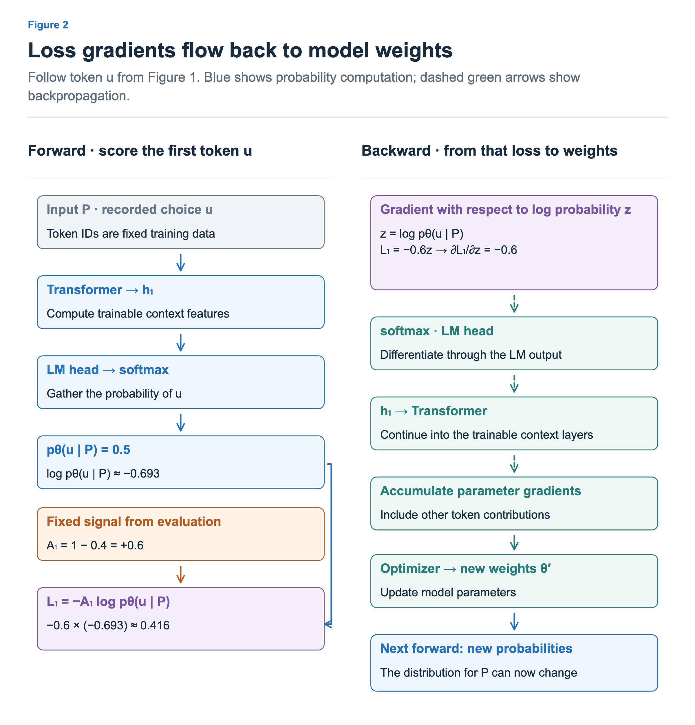
Figure 2 follows u, the first token in Figure 1. If we temporarily write the log-probability as z, then with A₁ = +0.6 the loss is L₁ = −0.6z. Increasing z by 0.01 decreases the loss by 0.006. The slope of the loss with respect to z is therefore −0.6. This is the calculation shown in the first backpropagation block.

Here, −0.6 is the derivative with respect to the log-probability z. The derivative with respect to the probability p itself is −0.6/p, which equals −1.2 at p = 0.5. Gradients with respect to model weights are not copies of these values: they result from applying the chain rule through the computation of the log-probability. Backpropagation proceeds through softmax, the LM head, and the Transformer, and the optimizer updates the trainable weights. We do not overwrite an entry in a probability table: the next forward pass computes a new distribution from the updated weights.

Aₜ is held fixed during this policy update. Even when a critic is trained, we do not let the policy loss arbitrarily increase Aₜ itself; the critic is trained separately using its prediction error.

Also, “the direction that increases the probability” describes the signal from this token’s term. In practice, losses from many tokens and responses are combined, and the same weights affect outputs in many contexts. We therefore cannot guarantee that every token with a positive advantage will have a higher probability after the overall update.

Probability Ratios When Reusing the Same Data

Producing new responses requires computation. It may be more efficient to use data that took effort to generate and score for multiple weight updates rather than just one. However, as soon as the first update is complete, the current model differs from the model that produced that data.

The value used to compare them is the importance ratio, or probability ratio rₜ. Here, we will call the policy at generation time old and the policy currently being trained current. The current model’s probability, written as pθ above, is written as pcurrent below.

$$r_t=\frac{p_{\mathrm{current}}\left(x_t\right|s_t)}{p_{\mathrm{old}}\left(x_t\right|s_t)}$$

If the probability at generation time was 0.5 and the current probability is 0.6, rₜ is 1.2. This means that the same token in the same context is now selected with 1.2 times the probability. If we use this data again in the next update, the denominator is still 0.5. Replacing the denominator with the current probability each time would lose the comparison with the policy that generated the data.

To explain the calculation, we will now use an objective to maximize instead of a loss to minimize. The loss used for training is the negative of this objective. PPO starts with a term that maximizes rₜAₜ, the probability ratio multiplied by the fixed advantage, and applies the clipping we will explain shortly. Simply multiplying the earlier −Aₜ log p formula by an additional rₜ would give a different derivative from the one used in PPO.

Why does rₜAₜ also contain the same learning direction as the log-probability? With the denominator and Aₜ held fixed, the gradient of rₜAₜ is rₜAₜ × the gradient of the current log-probability. At the starting point where the current policy equals old and rₜ = 1, this connects to the basic policy gradient we saw earlier. However, rₜ being 1.2 does not mean that the actual probability or weight change is exactly 1.2 times as large. The model’s gradients, the learning rate, and other samples also affect the result.

Here, we have assumed that generation and training perform the same probability computation. We will separately examine in article 9 how engines or quantization can produce different computed probabilities even with the same weights.

Clipping Stops Pushing Choices That Have Changed Enough

Adding a probability ratio does not automatically prevent large updates. If we keep increasing rₜAₜ when Aₜ is positive, there is still an incentive to raise the probability further for the same data even after it has already increased. PPO’s clipped objective limits this incentive.

First, we also compute a value with rₜ clipped to a specified interval. The figure below uses an interval from 0.8 to 1.2 for illustration. The notation is clip(input, lower bound, upper bound). We multiply the clipped ratio by Aₜ, compare it with the original term rₜAₜ, and maximize the smaller of the two.

Original term:    rₜ × Aₜ
Clipped term:     clip(rₜ, 0.8, 1.2) × Aₜ
Objective J:      the smaller of the two terms
Loss to minimize: −J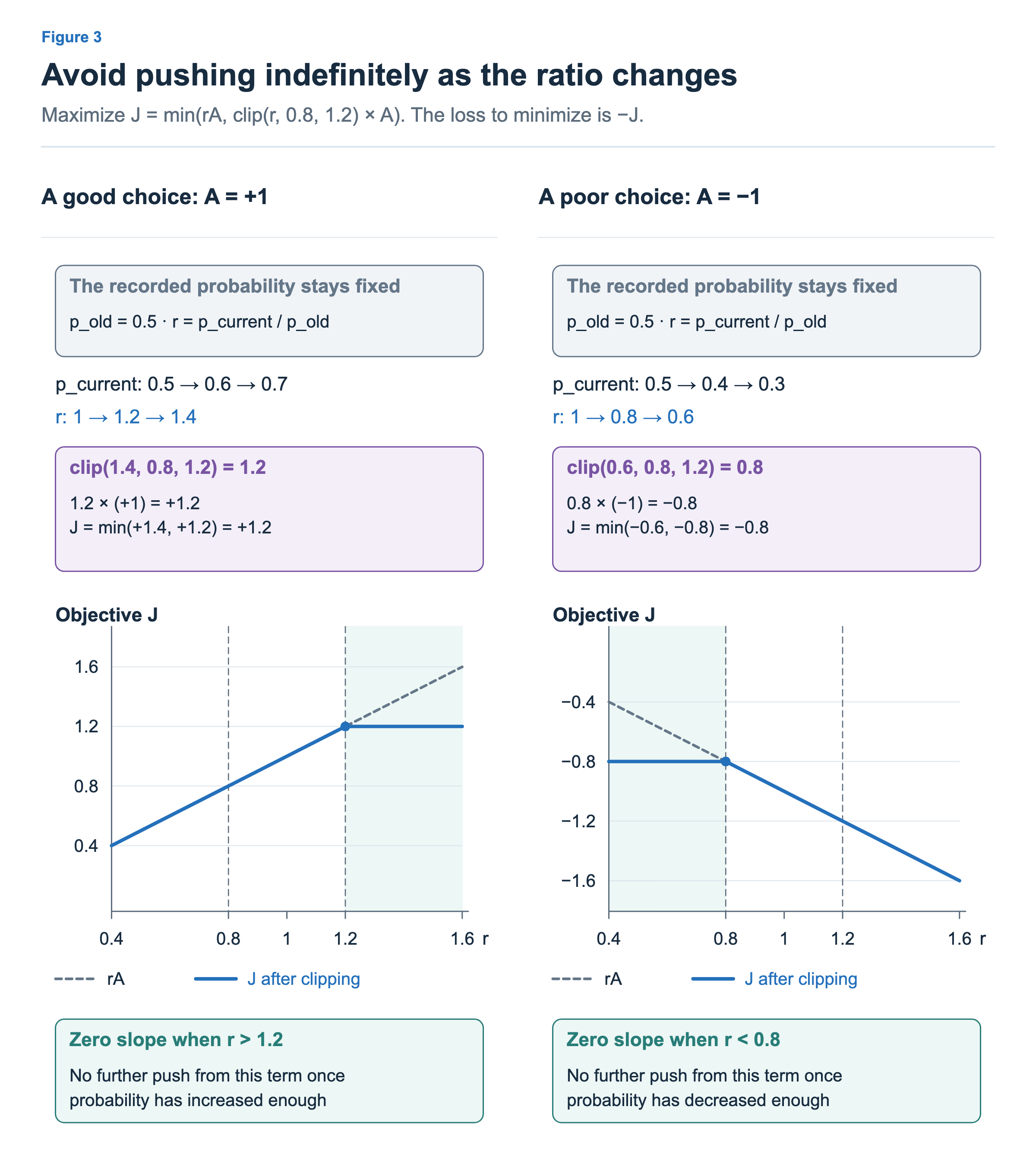

If Aₜ = +1 and rₜ is 1.4, the two terms are 1.4 and 1.2. We use the smaller value, 1.2. Even if rₜ increases further to 1.5, J remains 1.2, so this term alone provides no benefit from increasing it further. This is why the graph for positive Aₜ is flat in the region rₜ > 1.2.

When Aₜ = −1, the opposite side becomes flat. Clipping rₜ = 0.6 gives clip(0.6, 0.8, 1.2) = 0.8, which is still positive. Multiplying it by Aₜ = −1 gives −0.8. The original term is 0.6 × (−1) = −0.6, so J is the smaller of the two terms, −0.8. The vertical axis shows objective J, which includes multiplication by the advantage, rather than the probability ratio. This is why the values on the right are negative.

A negative objective can still be maximized. For example, as rₜ falls from 1 to 0.8, J increases from −1 to −0.8. But lowering rₜ further to 0.6 leaves J at −0.8. The probability of the unfavorable choice has already fallen enough, so we remove the incentive to push it down further.

Why, then, are both graphs not flat beyond both 0.8 and 1.2? The figure plots J, the minimum of the original and clipped terms, rather than the clipping result alone. When the probability moves in the wrong direction, the original term is selected.

If Aₜ = +1 but rₜ = 0.6, the probability of a good choice has fallen instead. The original term is 0.6 and the clipped term is 0.8, so J = min(0.6, 0.8) = 0.6. Flattening this region would also remove the signal to raise the probability again, so the slope is preserved.

If Aₜ = −1 but rₜ = 1.4, the probability of a poor choice has risen instead. The original term is −1.4 and the clipped term is 1.2 × (−1) = −1.2, so J = min(−1.4, −1.2) = −1.4. The signal to lower the probability again is preserved here too. The role of min is to remove the incentive to push further after sufficient movement in a favorable direction, while retaining the signal to reverse movement in an unfavorable direction. PPO §3

Clipping does not force the probability ratio itself to stay within 0.8–1.2. It changes the shape of the loss. Other samples and auxiliary losses can move the weights, so the actual probability ratio can lie outside the interval. Also, generating fresh data online does not mean that every RL algorithm must use the same clipping. It is one representative way to manage the relationship between the data and the current policy.

Separately Managing Deviation from a Reference Policy

How much the policy has changed since the data was generated and how far it has moved from a model we want to keep as a reference are different questions. For the latter, we can introduce a reference policy. For example, we can freeze the model at the start of RL and compare the current policy against it.

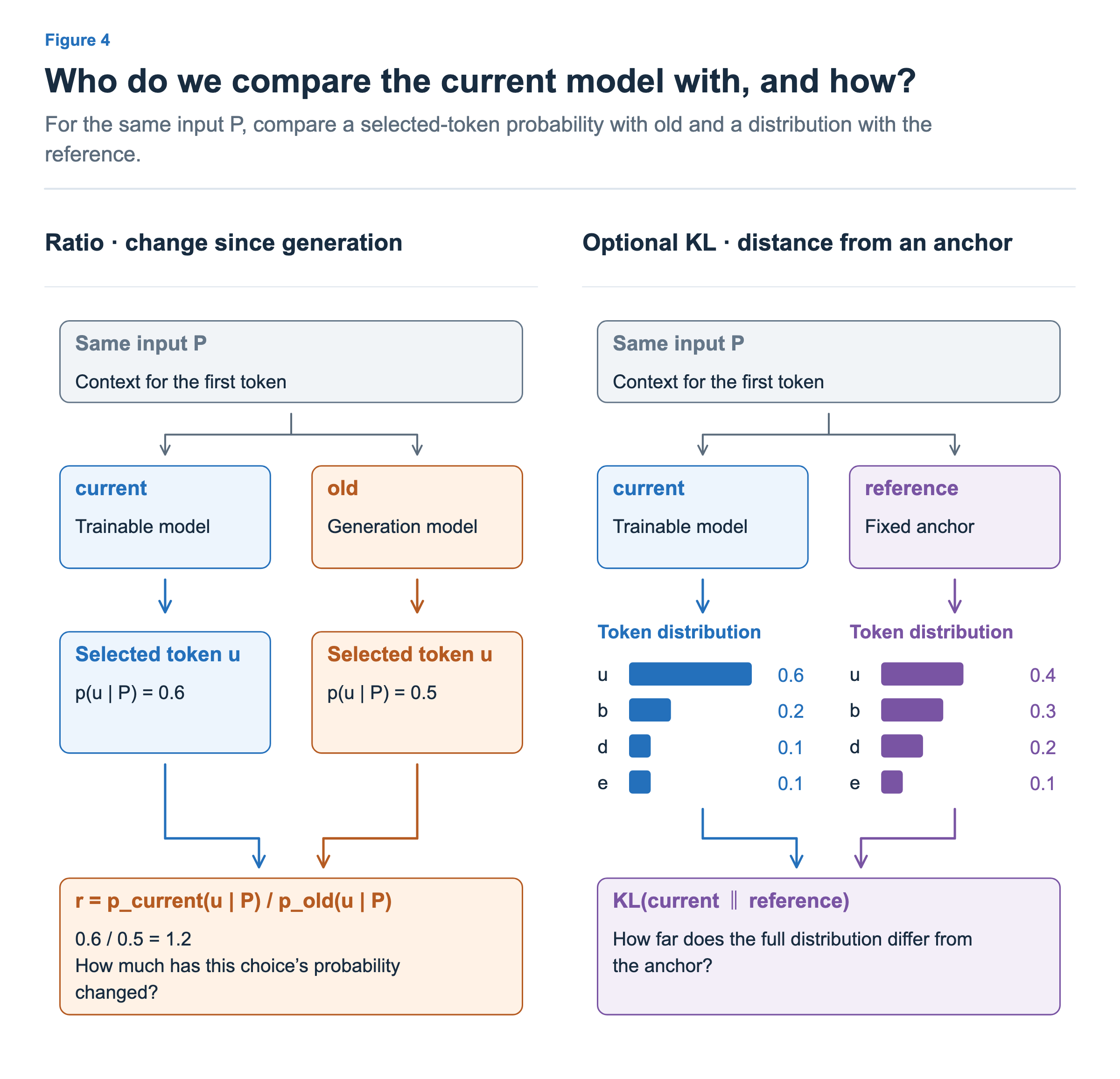
The left side of Figure 4 illustrates the selected token u changing from a generation-time probability of 0.5 to a current probability of 0.6. The right side assumes a vocabulary of just four tokens to draw the two distributions. Both current boxes represent the same current model. The boxes show model roles needed for comparison, not the number of physical servers.

We can regularize the difference between the probability distributions produced by the current and reference policies in the same context by measuring their KL divergence. When it is added as a separate loss, we minimize the policy loss plus β × KL. β sets the relative weight between changing the policy according to rewards and staying close to the reference.

Some training setups instead include the reference-policy KL as a penalty in the reward, allowing it to affect the advantages. We need to distinguish where it is added; not every setup adds it in both places at once. It is also possible to use a setup without a reference policy. RLHF Book — Regularization

Old and reference may initially have the same weights. As training progresses, however, old can change as it generates new data, while the reference in this example remains in its initially chosen state. We also do not need to run the old model every time we compare against it. We can record the selected tokens’ generation-time log-probabilities in the data and reuse them.

We can now see where the information originating from rewards leads. Rewards and a baseline produce advantages, while the current model’s probability computation provides a differentiable path from the loss to the weights. Probability ratios and clipping for data reuse, and KL for staying close to a reference policy, control different parts of this path.

In the next article, we will look more closely at the baseline that we have so far treated as a single box. We will start with comparing responses to the same question, then introduce a critic that predicts expected future rewards from each context.