Delivering New Weights to the Inference Engine

The system map in Article 6 had arrows in two directions. Generated experience goes to the learner, and trained weights return to the generator. This article takes a closer look at the second arrow: weight sync.

First, prepare the weights in the partitions and format expected by the inference GPUs. Next, choose a transfer path that fits the deployment and network. Finally, finish preparing the new weights for computation and handling existing requests and caches before resuming generation. Following these three stages—prepare → transfer → resume—shows why copying time alone cannot describe the cost of weight sync.

Adapting the same weights to different partitions

Imagine one weight tensor as a 4×4 matrix. The numbers 1–16 in the figure are educational values for tracking the positions of pieces. Training GPU 0 holds the two left columns, and GPU 1 holds the two right columns. Inference GPU 0 needs the two top rows, and GPU 1 needs the two bottom rows.

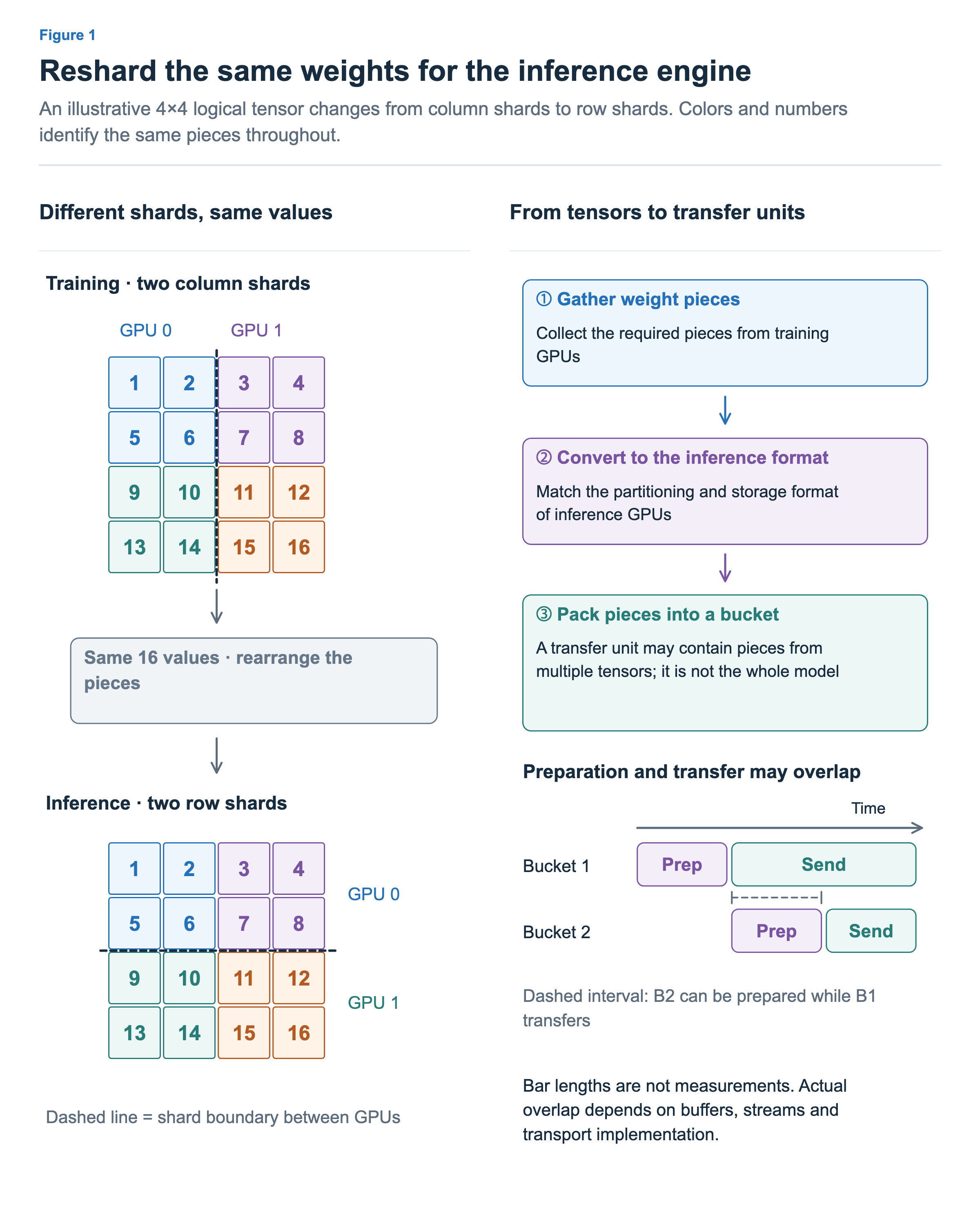
Consider the first row [1, 2, 3, 4] needed by inference GPU 0. [1, 2] is on training GPU 0, while [3, 4] is on training GPU 1. Copying the entire memory of either training GPU alone cannot assemble that first row. Pieces must be received from multiple locations and arranged in the order the inference side expects. This change in partitioning is called resharding.

Real models have many tensors and use various forms of parallelism. Tensor parallelism (TP) divides computation on one tensor across multiple GPUs, while expert parallelism (EP) distributes MoE experts. ETP also partitions tensors within an expert. When training and inference use different parallel configurations, the transfer process must reconcile them.

Miles’s Megatron path includes gathering the TP and ETP shards of individual weights and, when necessary, gathering experts distributed through EP. Gathering individual tensors in this way is different from gathering all weights onto one GPU at the same time. Weight sync does not require being able to hold the entire model at once. Miles v0.1.0 weight-conversion code

Tensor names, the layout of arrays that store multiple weights together, data types, and quantization metadata must also match the inference engine’s conventions. The quantized values and scales discussed in Article 8 are semantically linked. Transferring only the numeric array and applying the wrong corresponding scale or partition information does not transfer the same policy.

Grouping transfers and overlapping preparation

Starting a separate transfer for every small tensor can incur substantial repeated call overhead. A bucket is a transfer unit that groups multiple tensors or tensor pieces. The entire model does not have to form one bucket.

At the bottom of Figure 1, bucket 2 is prepared while bucket 1 is being sent. Overlapping preparation and transfer in this way can reduce the time spent waiting for sequential steps. However, it may require multiple buffers or create contention for the same memory and communication resources. Not every implementation overlaps work as shown in the figure or achieves the same benefit.

Larger buckets can reduce the number of calls, but may delay the first transfer and require more temporary memory. Smaller buckets are easier to send earlier, but may increase repeated overhead. Bucket size therefore needs to be considered together with the model and partitioning configuration being measured.

We must also distinguish transferring the model weights needed for inference from saving a checkpoint that can fully restore training. Information needed to resume training, such as optimizer state, is not necessarily part of ordinary inference weight sync.

Broadcast, P2P, and disk-delta paths

Miles v0.1 describes broadcast, P2P, and disk-delta as transfer methods for disaggregated deployments. The figure below shows the memory and storage through which values pass. A shorter line does not mean a faster path.

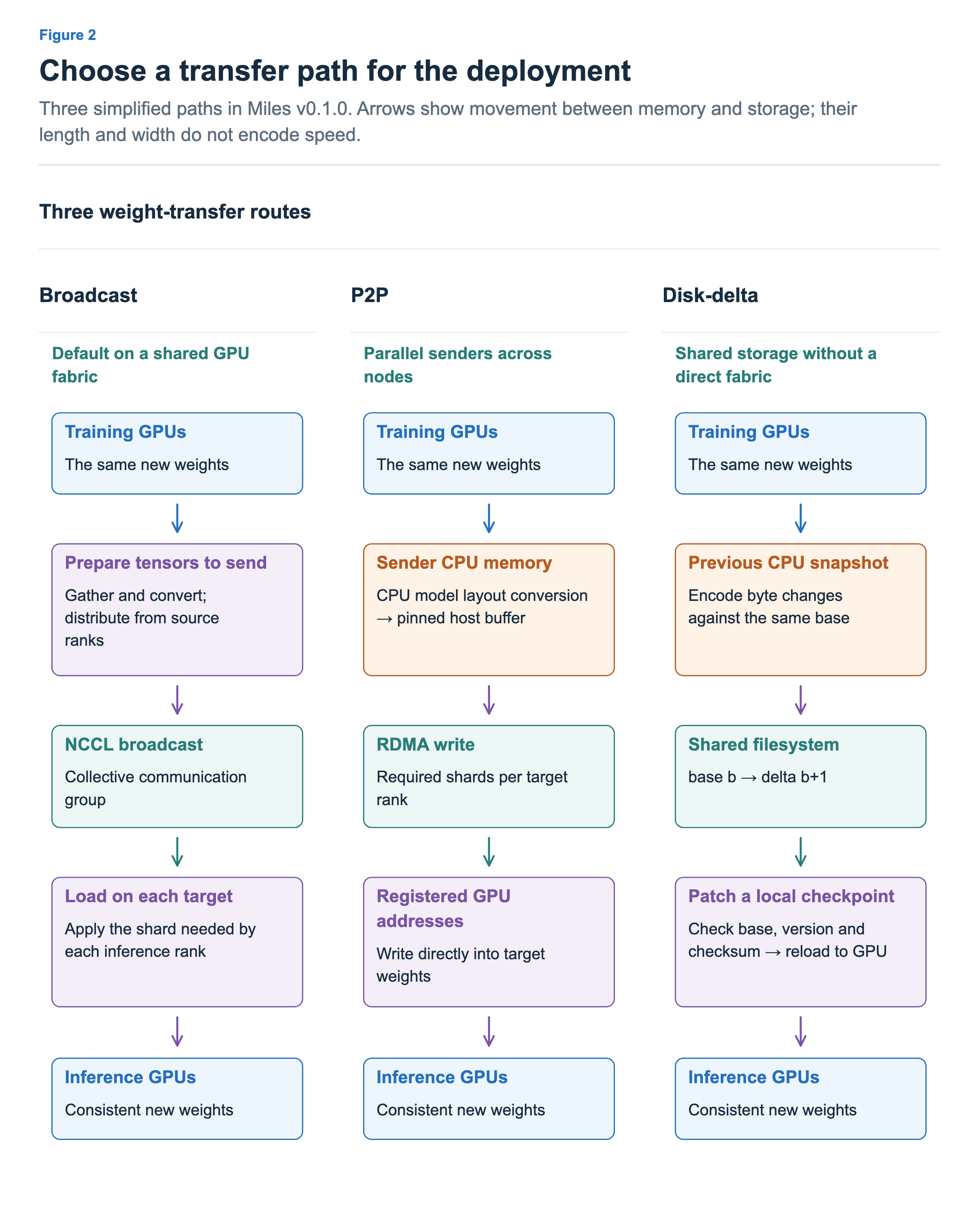
Broadcast distributes prepared weights to the participants in a communication group. NCCL is a library for collective communication in which multiple GPUs exchange data. After reception, each inference rank—a participating process in the distributed execution—applies the weights to its own partition. The actual source and communication-group configuration depend on the parallel layout.

P2P is a path configured to deliver the required pieces directly to their destinations. However, “specifying the destination directly” and “moving data only from GPU to GPU” are different things.

This Miles implementation applies weights from the training GPUs to a model copy in the sender’s CPU memory to convert them into the layout needed for inference, and uses pinned host buffers. Pinned memory is host memory fixed in place so its location remains stable during transfer. RDMA is a communication mechanism for directly reading from and writing to registered remote memory. The implementation then writes to the weight addresses of the target inference GPUs registered for RDMA. Therefore, part of the path passes through the sender’s CPU memory. Miles P2P documentation, sender code, SGLang receiver code

Using RDMA does not mean that CPU memory disappears from the entire path. The benefits and costs of this implementation must be assessed together with parallel transmission from the sources, layout conversion, preparation of transfer data in sender host memory, the network, and post-processing at the destination. Nor are we claiming that the receiver-code revision pinned here is the exact revision used in every performance experiment in the paper.

Disk-delta transfers change data through shared storage. Here, a delta is not the same concept as mathematically subtracting the old weights from the new weights. The Miles path encodes byte changes relative to a previous snapshot, applies them to a matching base checkpoint on the receiver, and then loads the result onto GPUs. If the base versions do not match, the change data alone cannot produce the correct new state. Miles disk-delta code

Even when parameter values change only slightly, how much their byte representation changes and how well it compresses are separate questions. We cannot assume that deltas are always small, and storage, reading, patching, and reload costs remain. This implementation can overlap receiving files and patching the local checkpoint with generation, and pauses generation before reloading the actual GPU weights. Generation therefore does not necessarily remain paused throughout the entire transfer.

When training and inference take turns using the same GPUs, other paths such as local transfer or IPC—memory sharing between processes—are possible. It is difficult to place them and the three methods above into one universal speed ranking. We also should not assume that other training backends, such as FSDP, support the same options as the Megatron path described here.

Choosing a transfer method for the environment

The choice depends not only on model size, but also on the number of nodes on each side and the available communication paths.

Method	When to consider it first
Broadcast	Default on a shared GPU fabric, especially with few nodes
P2P	Both training and inference span multiple nodes
Disk-delta	No direct GPU fabric, or full-weight transfer volume is a concern

The Miles paper reports that P2P was slower than broadcast on a single node, while its advantage grew as the number of nodes on both sides increased. Multiple senders can contribute bandwidth and avoid sending unnecessary shards. In a small deployment, CPU preparation costs may outweigh these benefits. These are observations under the paper’s measurement conditions, not a universal speed ranking. Miles v0.1, §4.2–4.3

Resuming generation with the new weights

Now suppose we switch from deployed version v20 to new weights v21. GPUs A/B participate in the same inference execution, and we assume this model requires requantization after receiving weights. The example below updates weights after winding down and stopping existing generation. It assumes that ongoing generation has been safely stopped or completed before the first change to the inference weights in use.

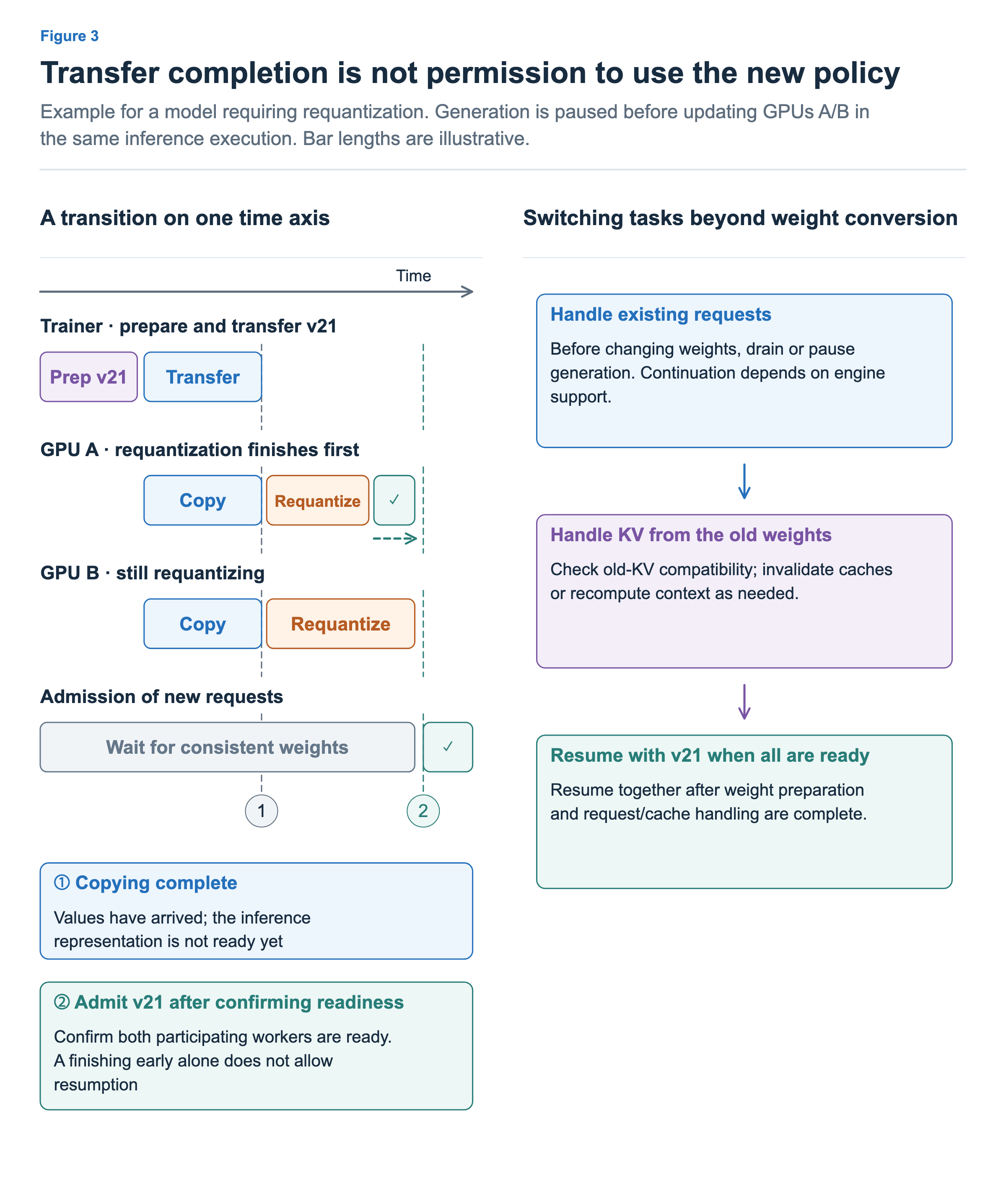
In the figure, copying finishes at the same time for A and B. A finishes requantization first, while B is still converting its weights. Under this transition protocol, generation does not resume across the system just because A is ready. The system checks that both GPUs participating in the same computation are ready to use consistent new weights.

Here, requantization rebuilds the received weights in the low-precision representation used by the inference kernel. The required quantized values, scales, and related data must be ready before that kernel can run. This is why values arriving on a GPU and the inference representation becoming ready can be different events. The Miles paper includes about 884ms of post-transfer GPU requantization in its Kimi K2 measurement. The bars illustrate the ordering; they do not reproduce that timing. Miles v0.1, Table 8

Not every model requires requantization after reception. Depending on the implementation, weights may also need to be rearranged or packed in the order expected by the inference kernel. If the sender has already completed that preparation, the receiver need not repeat it. The earlier preparation stage and this stage do not imply that the same conversion must always run twice.

Handling existing requests and KV caches is a switching task separate from converting the weights themselves. The right side of the figure shows what else must be checked before generation resumes. Merely changing the version string to v21 does not guarantee readiness, so admitting new requests must be tied to actual completion signals.

There are several options for ongoing v20 requests. We can wait for them to finish, abort and retry them, or continue partial generation in a supported way. In every case, the actual generation version must be recorded. If the policy changes midway through one response, finer-grained version records may be needed, as discussed in Article 10.

KV computed with the previous weights also needs attention. Identical tokens do not mean that new weights can unconditionally be used with old KV. Which caches to invalidate and which contexts to recompute must follow the engine’s update protocol. We cannot assume that every system clears its entire cache in the same way.

We can also consider configurations that transition workers one at a time rather than stopping the entire fleet at once. Such configurations must manage which requests run on which consistent set of workers at which version. The figure does not prescribe all of those deployment methods; it illustrates the condition that generation must not start in an intermediate state where only some tensors have been updated.

Considering sync frequency and total time together

Frequent weight transfers make it easier for the generator to use a more recent policy, but incur conversion, communication, and resumption costs more often. Less frequent transfers reduce those costs, while potentially increasing the difference between the policy being trained and the generation policy. This connects to the same decisions as staleness management in Article 10. We must also check whether the configured update interval is measured in rollout iterations or actual optimizer updates. Those counts are not automatically the same unit.

If a large model is transferred after every short training update, weight sync may take longer than the update itself. This is conditional on the amount of training computation, transfer size, GPU and node placement, and network. We cannot declare in advance that generation always takes the longest or that one transfer method is always the fastest.

Measurement needs to include not just transferred bytes, but also resharding and format conversion, actual data movement, application and post-processing, and confirmation and resumption. If recomputing KV slows down the first request, that cost also needs to be observed. If pure network transfer becomes faster but overall RL does not, we can check whether the cost has moved to another stage.

Once the new weights are applied to the inference engine, experience generation can begin again. This cycle of generating experience, learning from rewards, and transferring new weights brings the series to a close. Looking at both the computations within each stage and how experience and weights move between engines helps us understand the overall flow of an RL system.