LLM RL in Review: From Token Choices to the System Loop

LLM RL evaluates responses produced by a model and uses that experience to change its future choices. The first half examines how token probabilities change. The second half examines how two engines divide up that computation.

This article brings together figures from Articles 1–13 for a roughly 30-minute presentation that you can follow by scrolling. The plan allocates about 16 minutes to learning principles, 12 minutes to systems, and 2 minutes to closing. Figure numbers retain their original numbering; the links in each section lead to fuller explanations.

An LLM acts by choosing the next token

In conventional RL, a policy observes the current situation and chooses an action. For an LLM, the prompt and preceding tokens are the situation, and choosing the next token is the action. The chosen token becomes part of the context for the next choice.

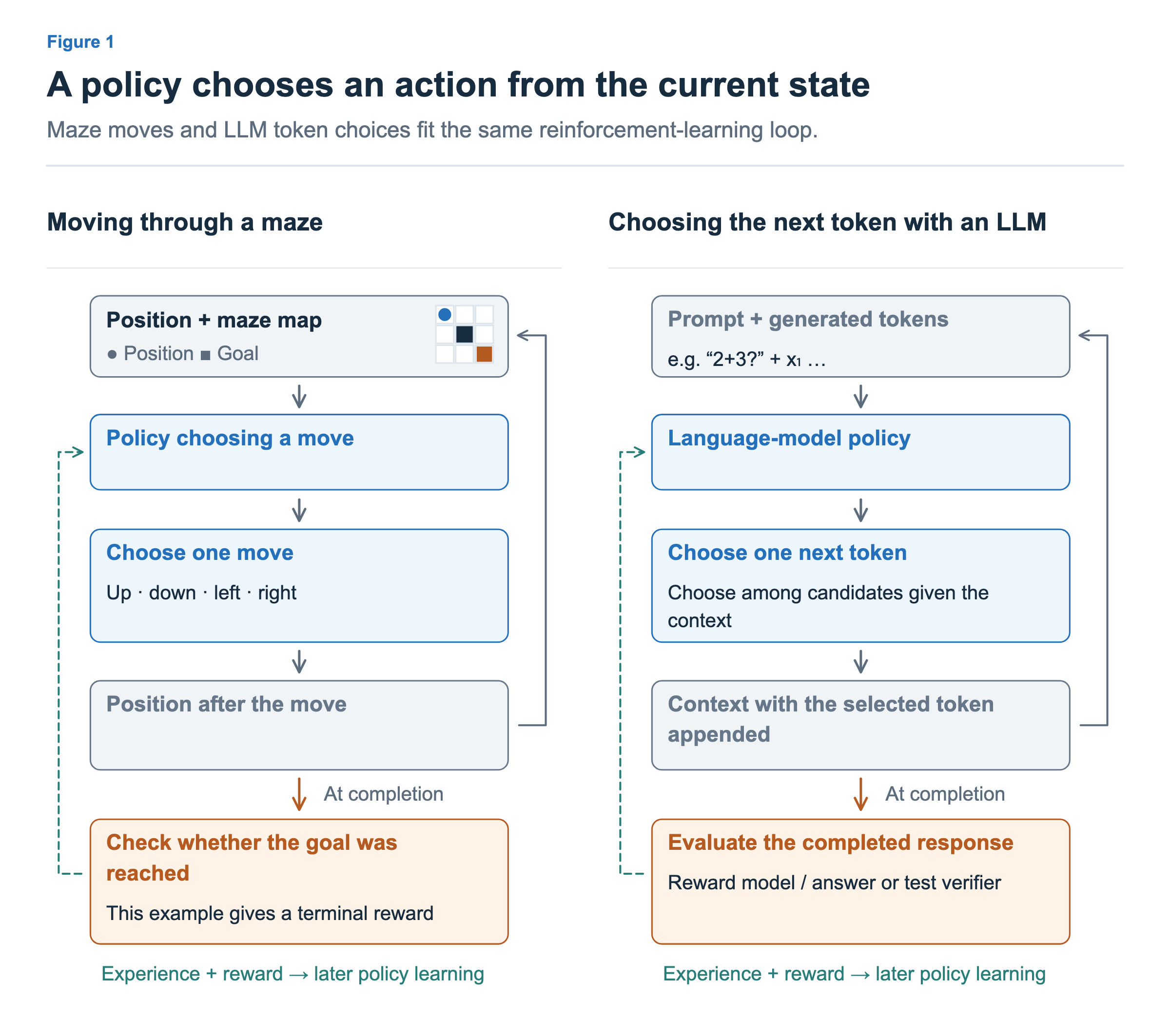
In a maze, the policy observes the current position and map, chooses a move, and changes position. An LLM observes the question and generated tokens, chooses the next token, and extends the context. Both examples evaluate the completed outcome and use experience and reward to train the policy afterward.

In a maze, the new position becomes the input to the next choice. For an LLM, it is the extended token context. Let us now unfold how token choices lead to a response and a reward.

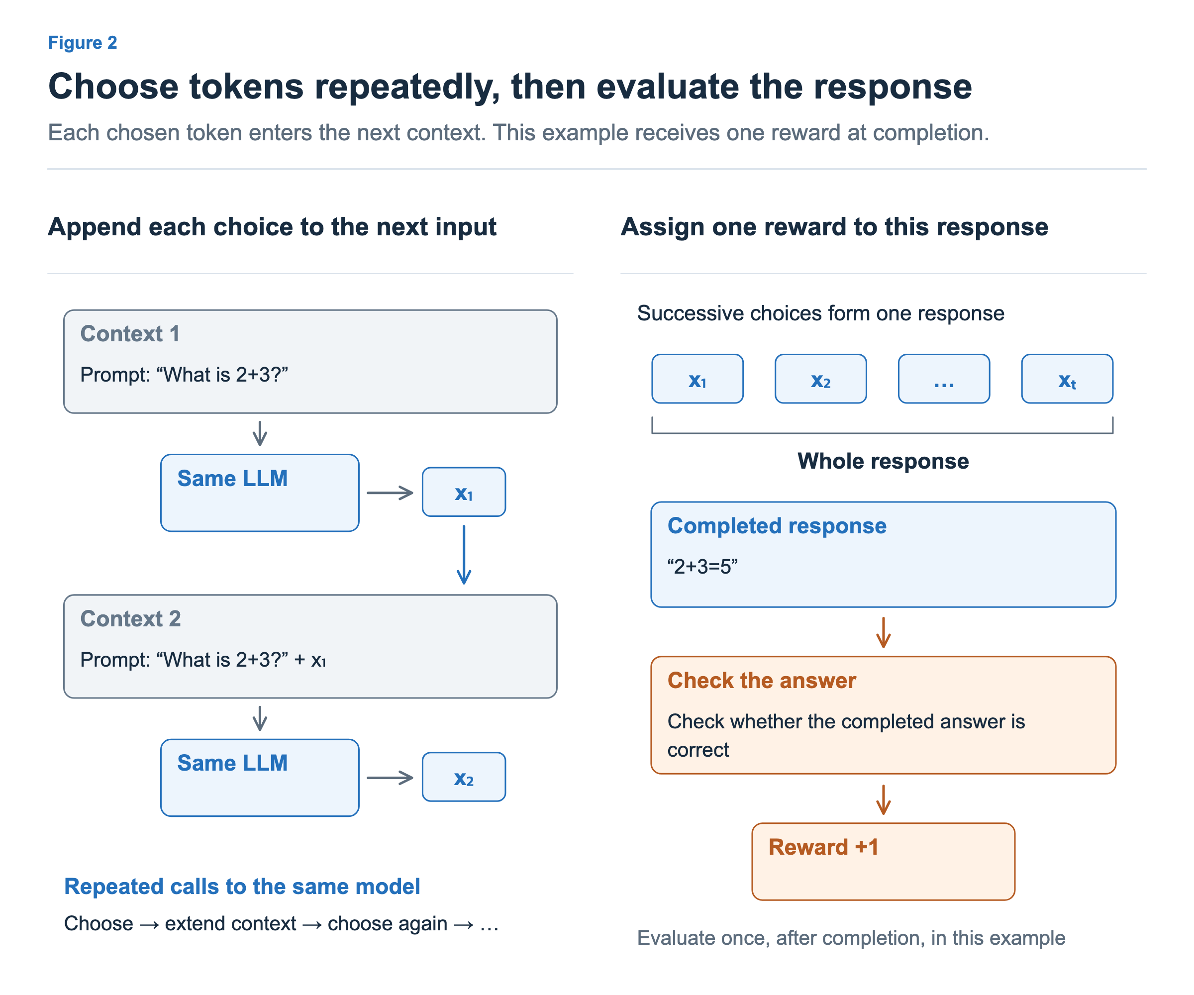
The same LLM selects x1 from the question, then selects x2 from the context containing the question and x1. Repeated choices complete the response 2+3=5. The response receives a reward of +1 once after its answer is verified.

Multiple choices form a response. We can verify its result by checking an answer or running code, or score it with a reward model or an LLM evaluator. This example gives one reward to the completed response, but learning returns to the token choices that produced it.

Article 1: Token generation and rewards

Learning changes the probabilities of recorded choices

Read the recorded response with the current model

If the generated response was u → b → d, we hold that record fixed during training. Instead of sampling a new answer, we compute the current model’s probability for the token actually chosen in each context.

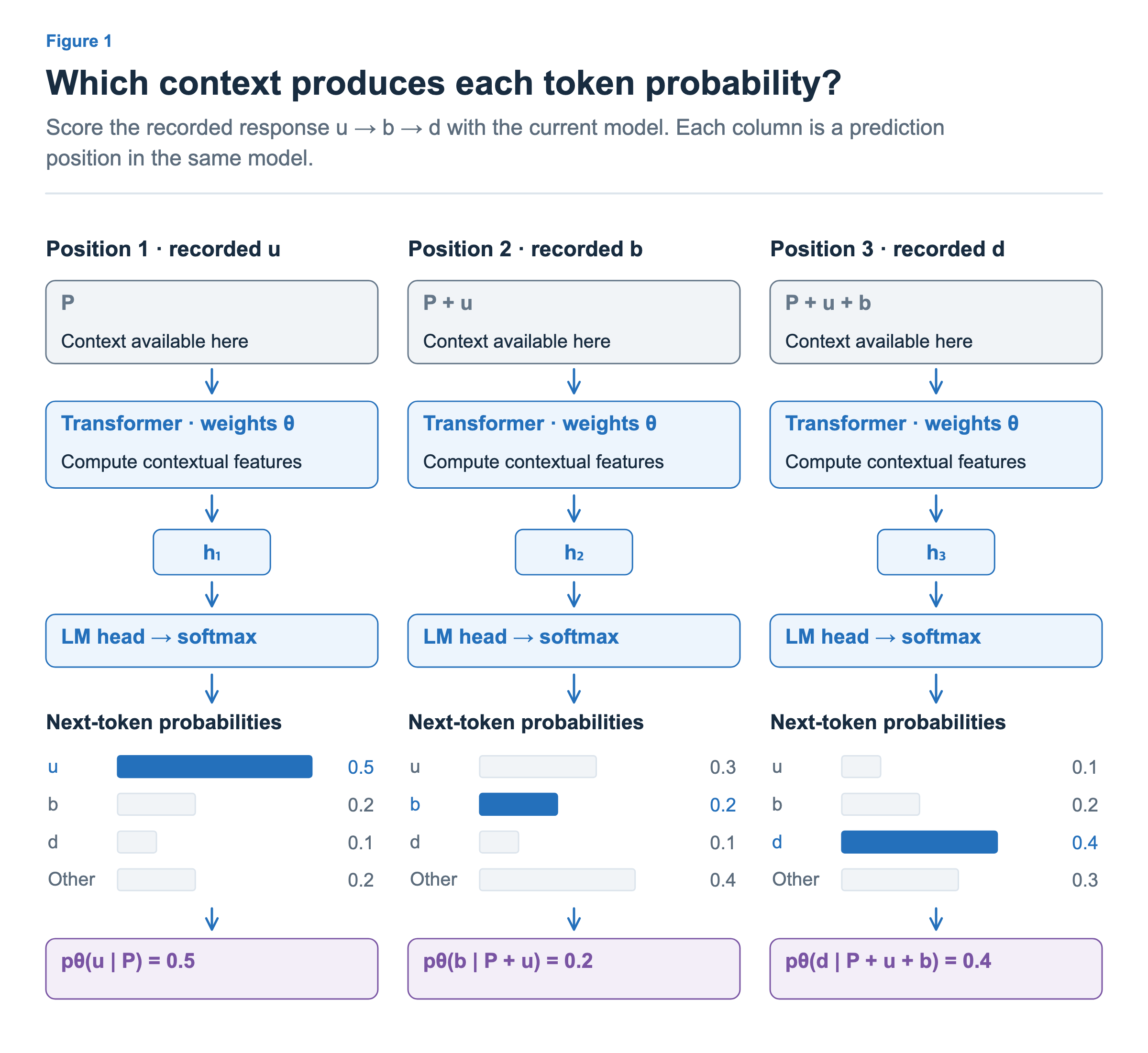
The same Transformer receives P, P plus u, and P plus u plus b at three prediction positions. Context representations pass through the LM head and softmax. The probabilities gathered for recorded tokens u, b, and d are 0.5, 0.2, and 0.4.

The probability of u comes from prompt P; the probability of b comes from P followed by u. The three positions in the figure are different prediction positions of the same model. During training, a causal mask lets us compute probabilities at multiple positions in one forward pass.

Advantage gives a direction; backpropagation changes weights

Advantage A is a signal indicating how much better an outcome was than a comparison baseline. In the simplest policy-gradient example, the loss is −A × log p(chosen token | context). Positive A pushes toward choosing that token more often; negative A pushes toward choosing it less often.

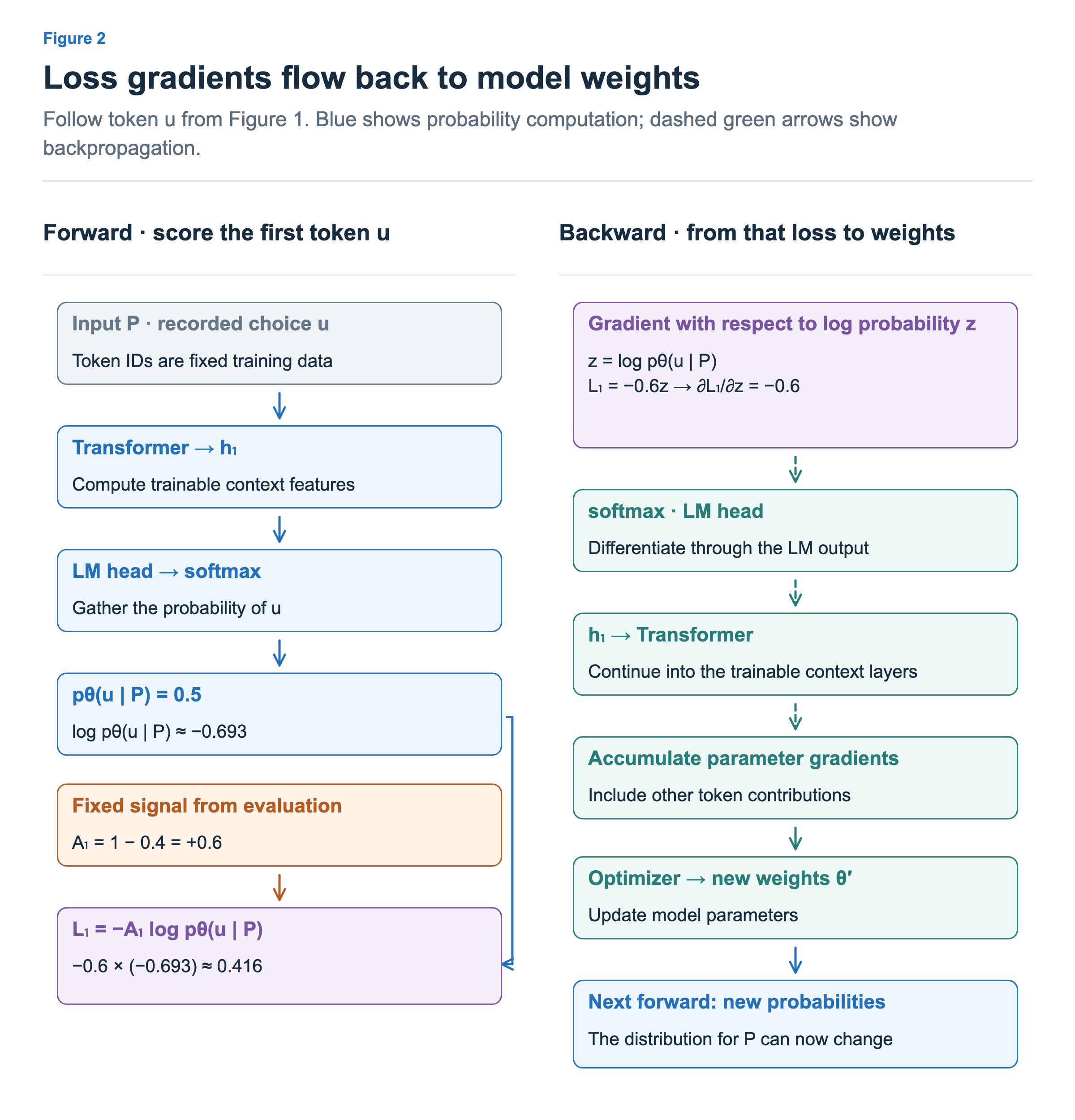
A return of 1 obtained from rewards minus a baseline of 0.4 gives an advantage of +0.6. The recorded context and selected token are fed into the current model to compute the log-probability. The fixed advantage and log-probability are used to compute a loss and backpropagate to the model parameters.

A is +0.6 in the figure, so the loss as a function of log probability z is −0.6z, whose derivative is −0.6. This gradient flows back through the LM head and Transformer to the weights. We change weights rather than editing a probability table directly; probabilities change in the next computation. Because multiple tokens share the same weights, each token’s probability is not guaranteed to move in the direction of its individual signal.

The behavior model and reference model have different roles

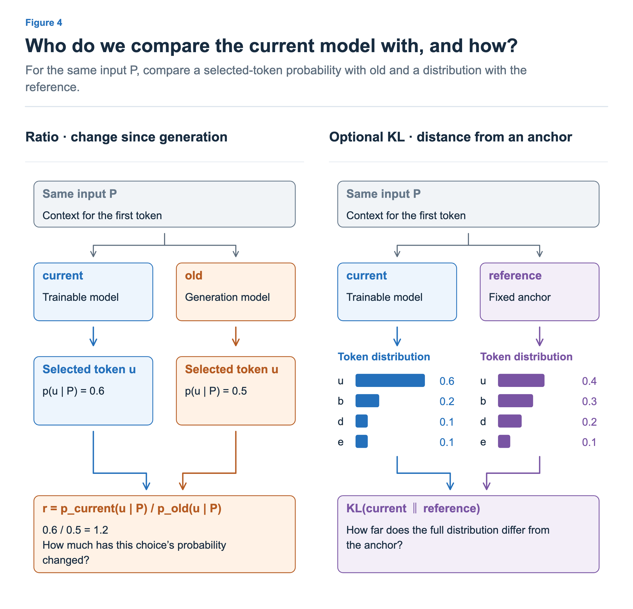
Each model receives the same input P. On the left, probabilities of 0.6 from current and 0.5 from old for selected token u give r=1.2. On the right, KL compares four-token distributions from current and reference. Both current boxes denote the same model.

The current model is the model being trained. A probability ratio compares it with the model that generated the data, using the same token, to account for changes since generation. PPO-style clipping stops the same data from continuing to push a choice that has already changed sufficiently in the favorable direction. A KL term against a separate reference model controls departure from a policy we want to stay close to; its use is optional.

Article 2: Probabilities, loss, and backpropagation

Comparing rewards determines which probabilities to raise or lower

Compare with other responses in the group

If four responses to the same question receive scores of 1, 1, 0, and 0, their mean is 0.5. A basic GRPO example compares rewards within this group. The example below also divides by the standard deviation, giving +1 to successes and −1 to failures.

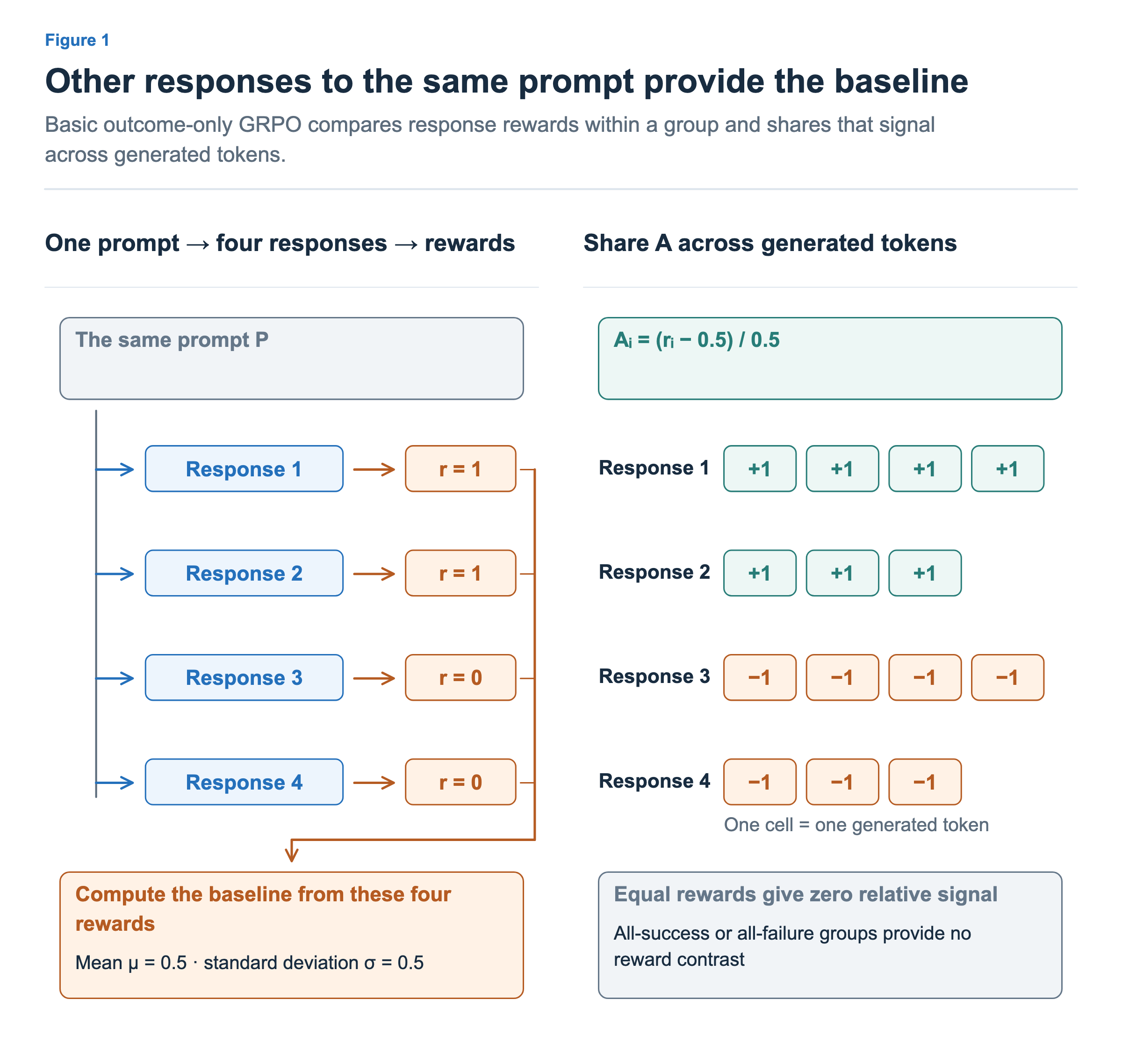
Four responses generated for the same question receive rewards of 1, 1, 0, and 0. Normalizing with a mean of 0.5 and a population standard deviation of 0.5 gives +1, +1, -1, and -1. Each response’s generated tokens use the advantage shared by that response.

In this setup, which uses only the response’s final reward, the same A is passed to every generated token in that response. This does not mean all tokens contributed equally to success. If all rewards are equal, the group’s relative reward signal disappears.

Compare with what was expected from that context

A critic predicts future rewards from the context before each token is chosen. Comparing the actual outcome with that prediction can produce a different comparison signal at each position, even with the same final reward.

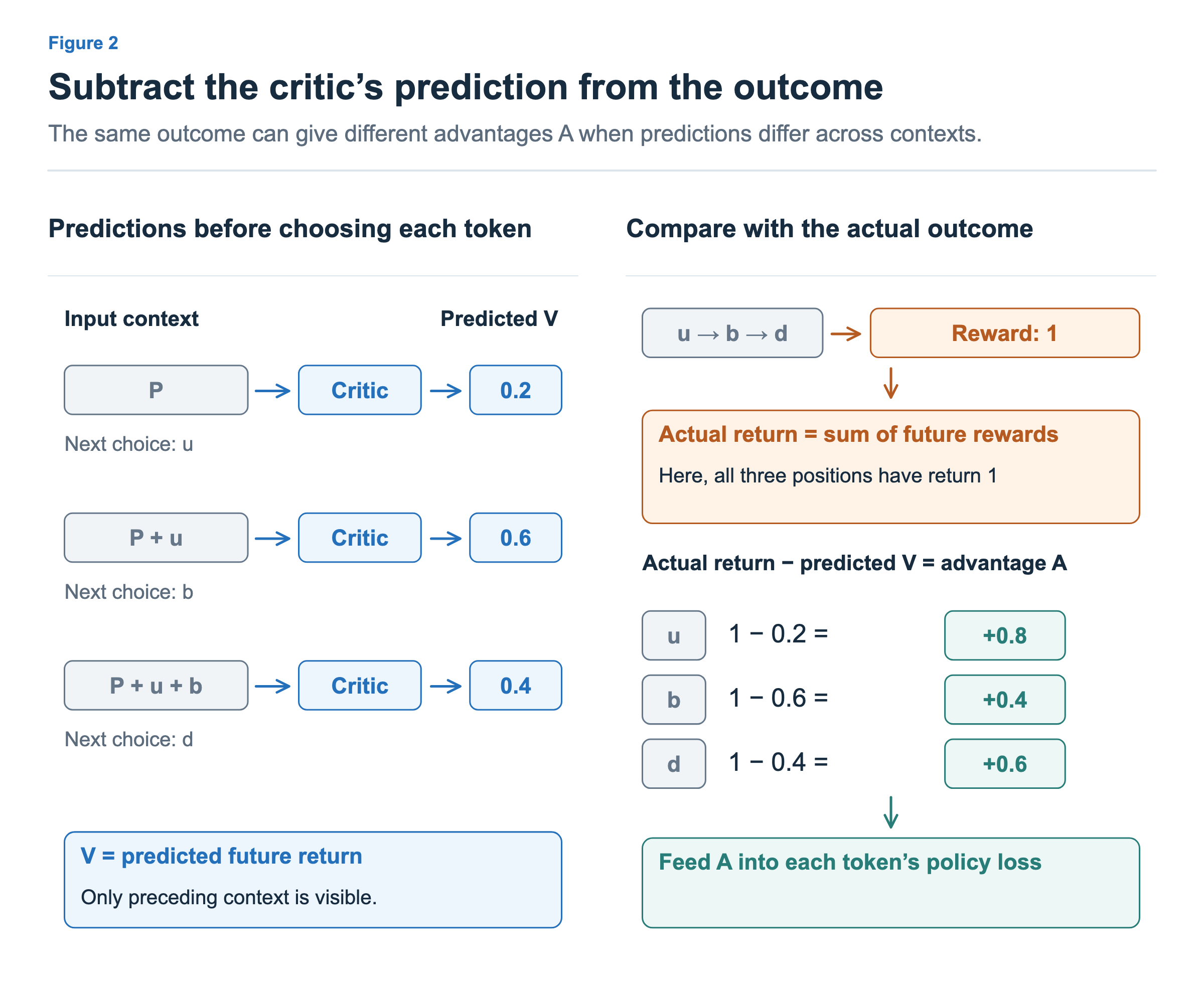
For contexts P, P+u and P+u+b, critic predictions are 0.2, 0.6 and 0.4. Subtracting each prediction from actual return 1 gives advantages A of 0.8, 0.4 and 0.6 for tokens u, b and d. Each A enters that token’s policy loss.

The figure is a simple example that subtracts a prediction from the fully observed return. In practice, PPO can use GAE, which combines TD errors. Group comparison uses other responses as its baseline; a critic uses a learned prediction. The choice of baseline also changes the cost of additional model computation and which experience must be awaited.

Article 3: Group comparisons and critics

A teacher provides learning signals in student-generated contexts

Learn along the paths the student actually visits

SFT learns the next target token from the preceding part of a provided answer. OPD obtains teacher signals in contexts generated by the student itself. Even when the student makes a choice that differs from the target path, it can learn in the resulting context.

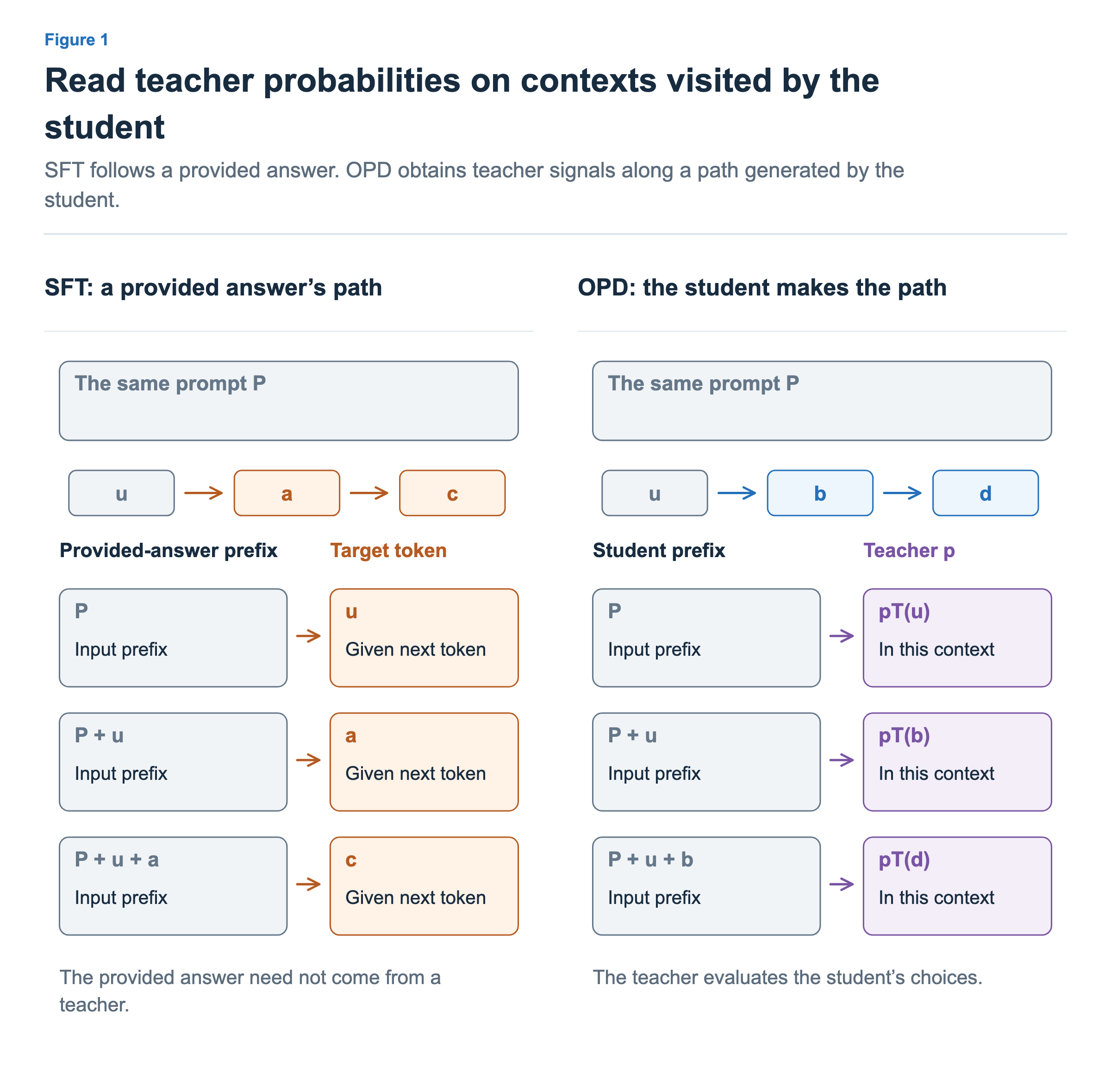
SFT learns the next target token in the contexts of the provided answer u, a, c. OPD reads the teacher’s token probabilities in the contexts of the student-generated path u, b, d. The third evaluation context also follows the student’s path, P+u+b.

Compare the probability of the same token in the same context

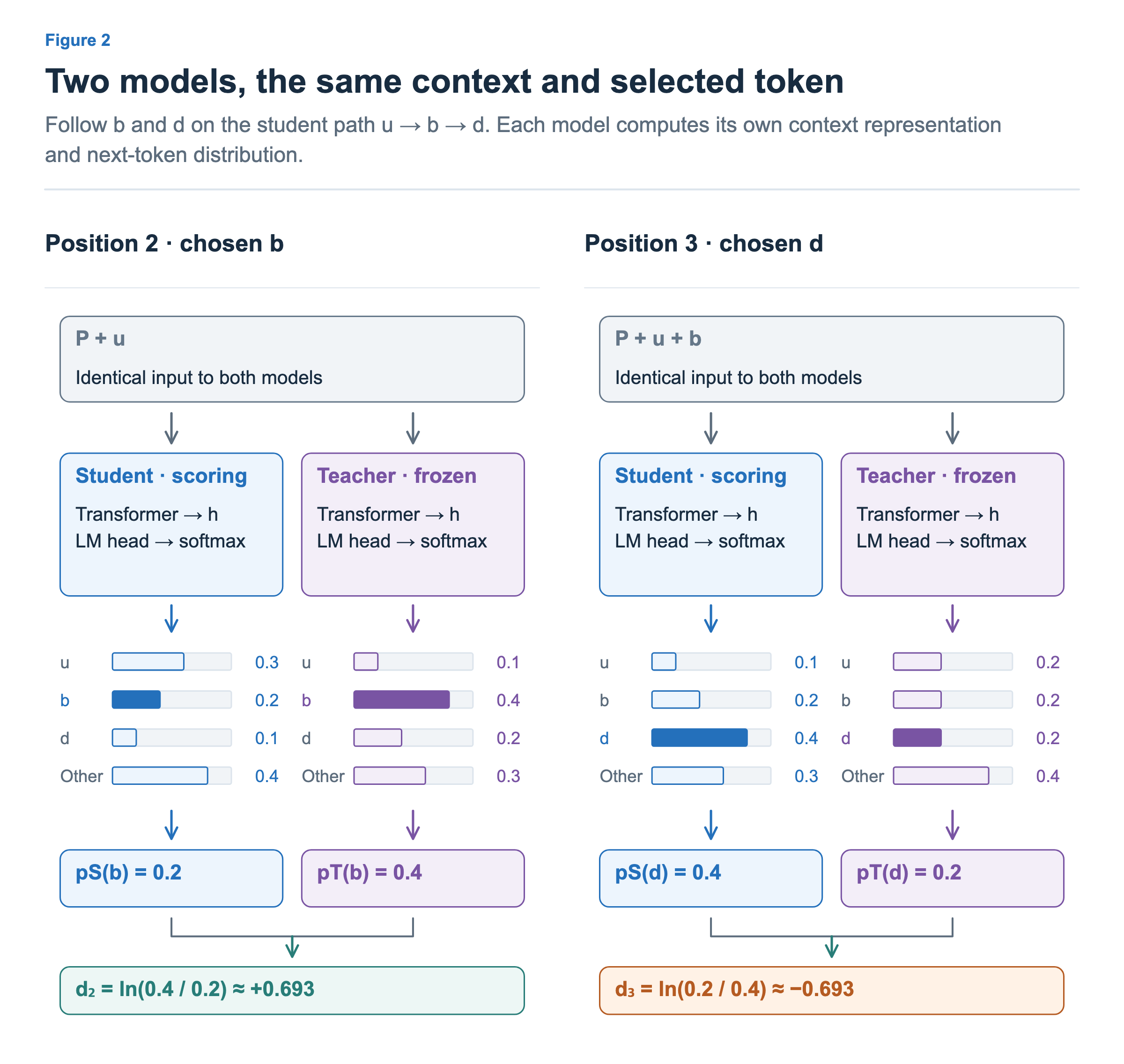
At P+u, two model forwards give probabilities 0.2 and 0.4 for chosen token b, producing +0.693. At P+u+b, student and teacher probabilities for chosen d are 0.4 and 0.2, producing -0.693. The signal-side probabilities are fixed for the update.

If the student gives probability 0.2 to its chosen token b and the teacher gives 0.4, the log-probability difference is ln(0.4/0.2), which is positive. Reversing the probabilities makes it negative. The OPD setup introduced here uses this teacher signal as a token-level learning signal.

We can add the teacher signal to advantages derived from task rewards, or use teacher signals without task rewards. A critic predicts future rewards; a teacher provides a next-token distribution. Although their signals come from different sources, they connect to a policy update that changes the student’s weights.

Article 4: Student contexts and teacher signals

The order of RL and OPD depends on the learning objective

A starting policy must be able to produce useful learning experience

To reinforce good choices using rewards, we need opportunities to observe useful differences within a limited generation budget. In the group-comparison example below, a mix of successes and failures provides a task-reward signal that an all-failure group does not.

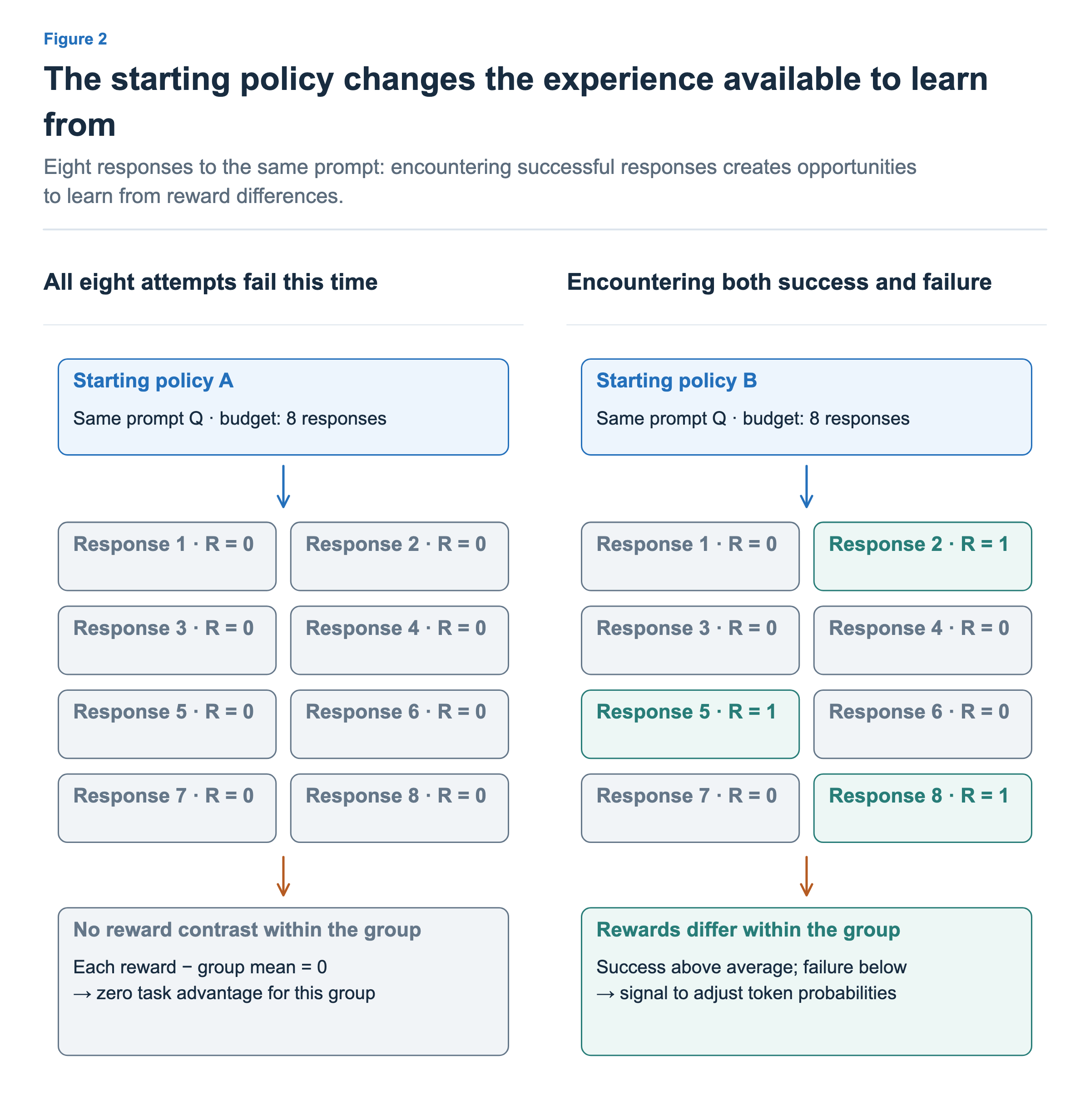
Eight responses are generated for the same prompt. If all rewards are zero, basic GRPO has zero group-relative signal. Mixed zero and one rewards allow different probability adjustments relative to the mean. These are hypothetical samples, not measured results.

Pretraining can build a foundation of language and knowledge, while SFT can establish a starting point through demonstrations. OPD can also improve the student’s behavior distribution before subsequent RL. The figure shows one case with equal group rewards; it does not imply that all RL requires successful responses to learn.

Develop specialist abilities and bring them into one student

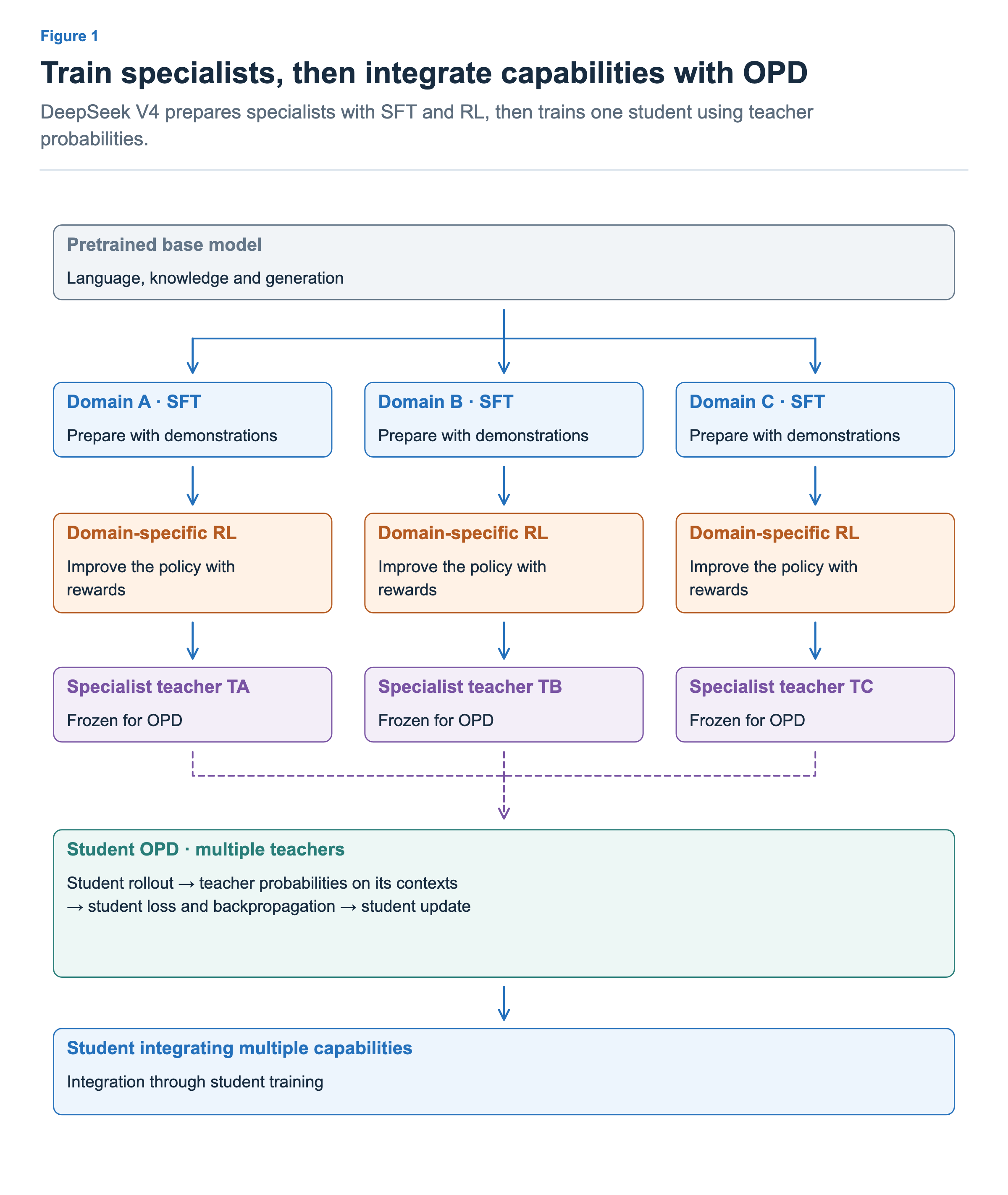
DeepSeek V4 illustrates a workflow that prepares specialist teachers through domain-specific SFT and RL, then trains one student from multiple teachers’ signals. It connects developing capabilities through rewards with transferring those capabilities to a student.

Domain-specific SFT and RL prepare specialist teachers from a pretrained model. Teachers provide probability information on student contexts, and OPD trains one student. Solid lines show model training; dashed lines carry teacher information.

Integrating capabilities and preparing for further learning are different goals

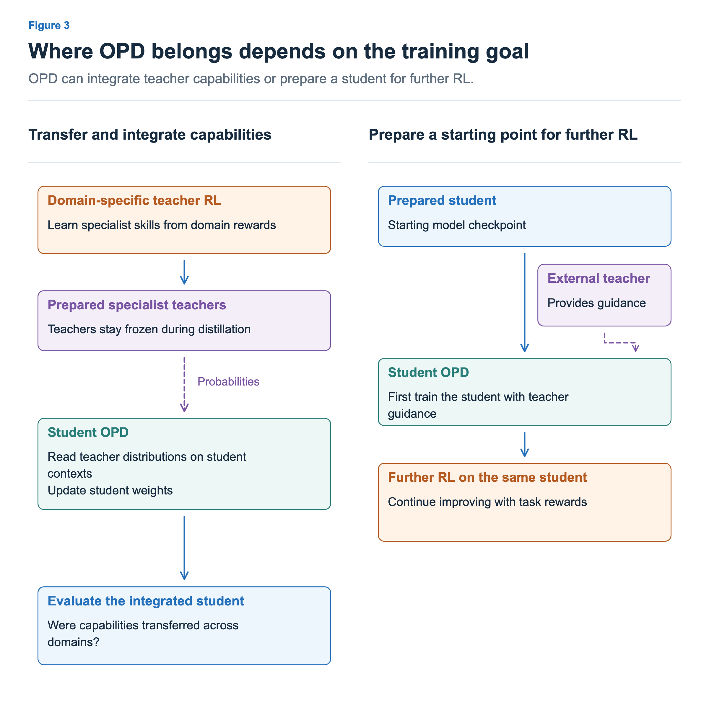
One path transfers capabilities through student OPD after teacher RL and then evaluates the student. The other trains a student through OPD and then applies task-reward RL to that same student. RL trains different models in the two paths.

Placing OPD after RL can integrate teachers’ capabilities. Placing OPD before the student’s RL can prepare its starting point for learning.

Choose both the teacher and the student’s starting context

MiMo V2.6’s MOPD² (Multi-Prefix Multi-Teacher On-Policy Distillation) uses multiple teachers while also choosing the dialogue contexts from which the student starts generating. It combines full rollouts starting from a question with new single-turn continuations from intermediate histories in teacher rollouts or SFT data.

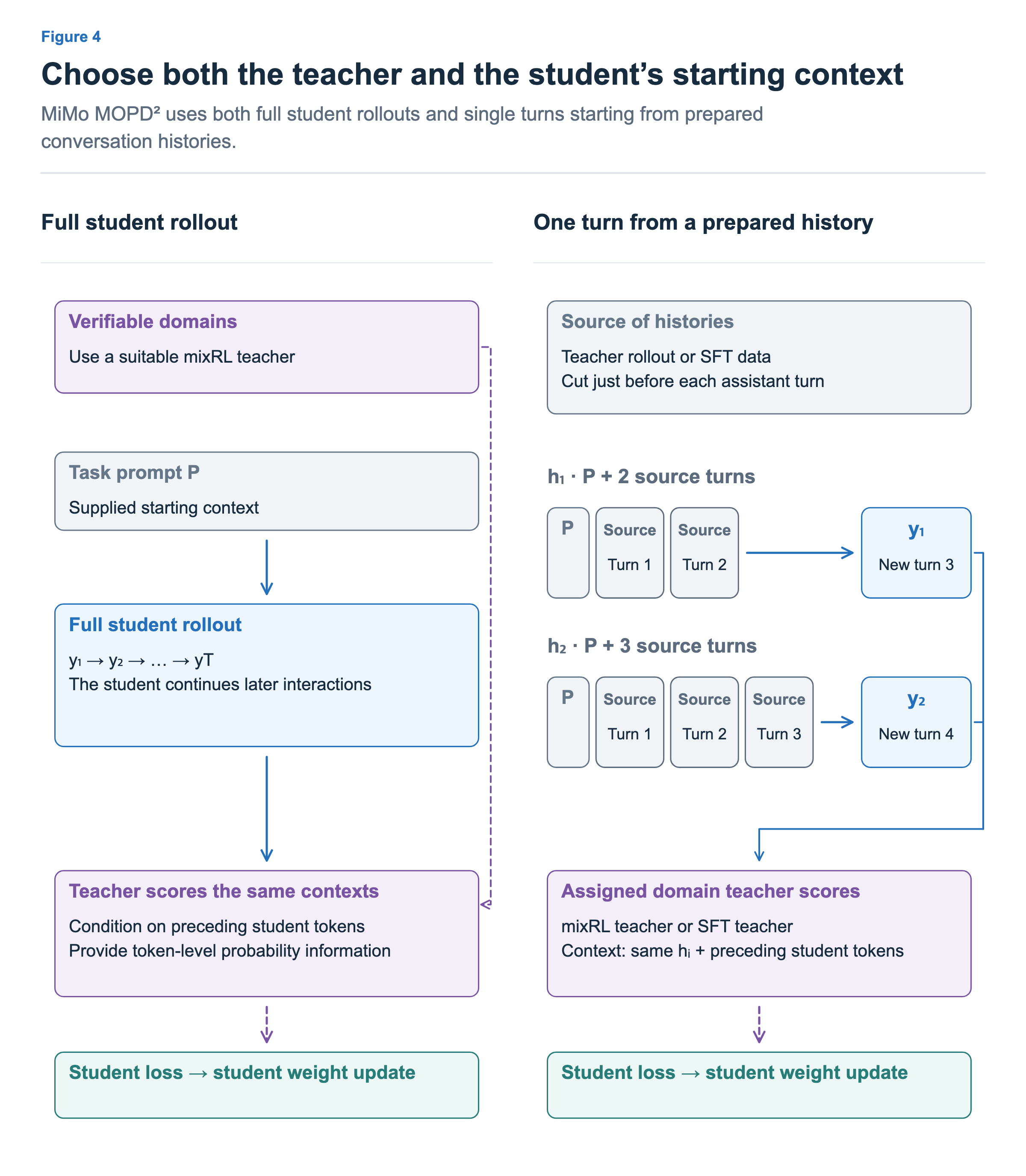
MiMo MOPD² uses full student rollouts from a prompt and independent fresh turn 3 (y1) from h1 with P and two source turns, and fresh turn 4 (y2) from h2 with P and three source turns. An assigned teacher conditions on the same context to provide probability information, and the student is updated.

For example, the student generates a new third turn from P + two original turns, and a new fourth turn from P + three original turns. These are independent starting points: the new third turn generated in the first example is not appended to form the second starting point. The assigned teacher sees the same context as the student and provides probability information. Rather than copying the original answer, the student learns by generating in multiple prepared contexts.

This illustrates that we can design not only the order of training, but also which teacher and which context the student learns from. MiMo V2.6 §5.6

Article 5: Combining RL and OPD, with sources

Experience moves to the learner; new weights move to inference

Let us place these computations in an execution system. The inference engine produces responses and tool-use experience. The training engine uses those records to compute probabilities and losses, then updates the weights.

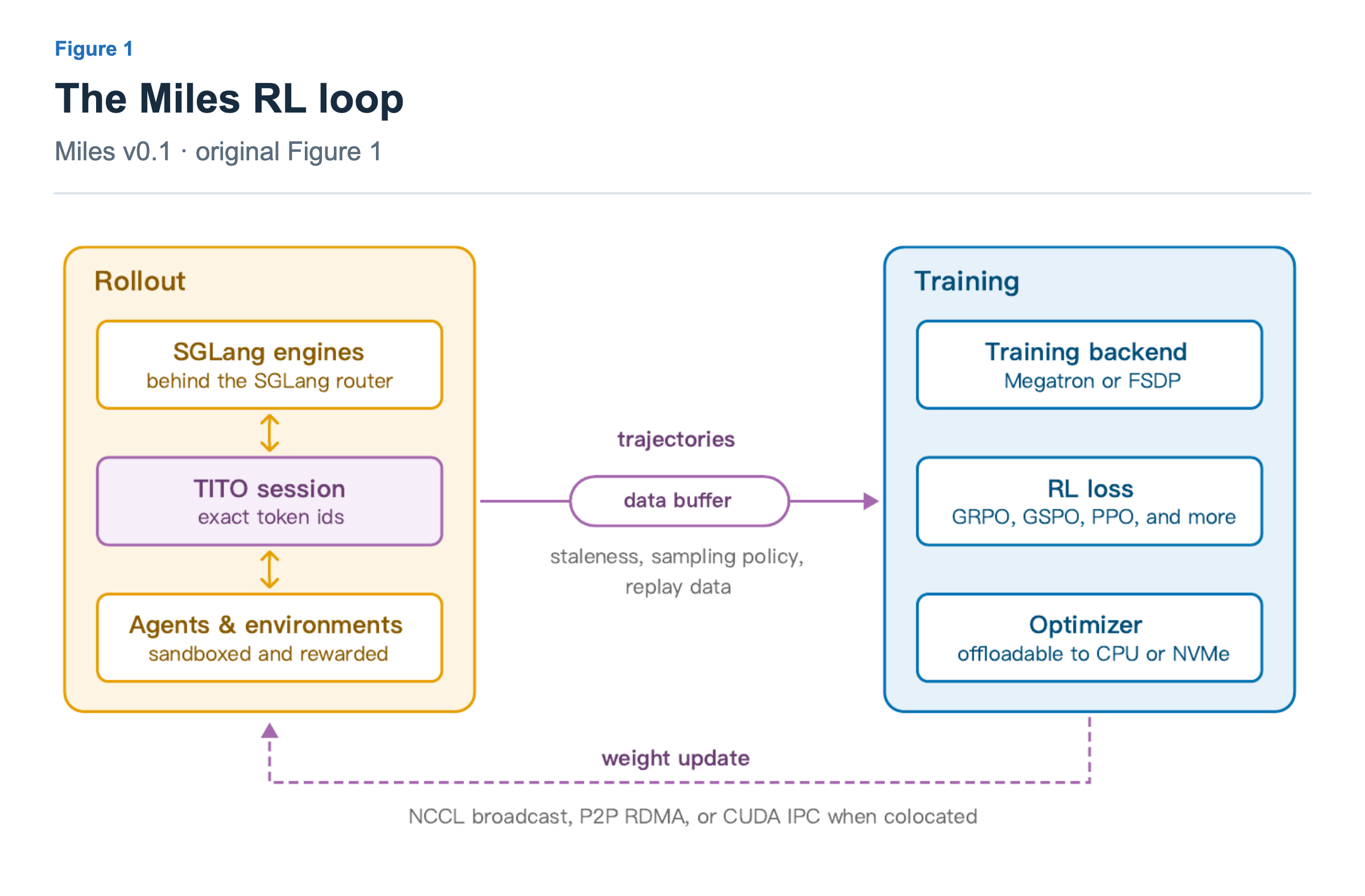
The RL loop from the Miles paper. Trajectories move from the SGLang inference engines on the left through a data buffer to training on the right. The lower weight-update path returns new weights to rollout.

Experience needs more than response strings: it also includes token IDs, generation-time log probabilities, rewards, masks marking the positions to train on, and policy versions. Updated weights travel in the opposite direction. We can read frameworks such as Miles, Slime, and NeMo-RL through these two arrows: experience transfer and weight synchronization.

Article 6: A map of the two-engine system · Figure source: Miles v0.1, Figure 1

Match the generation computation as closely as possible during training

Carry over token identities and expert choices

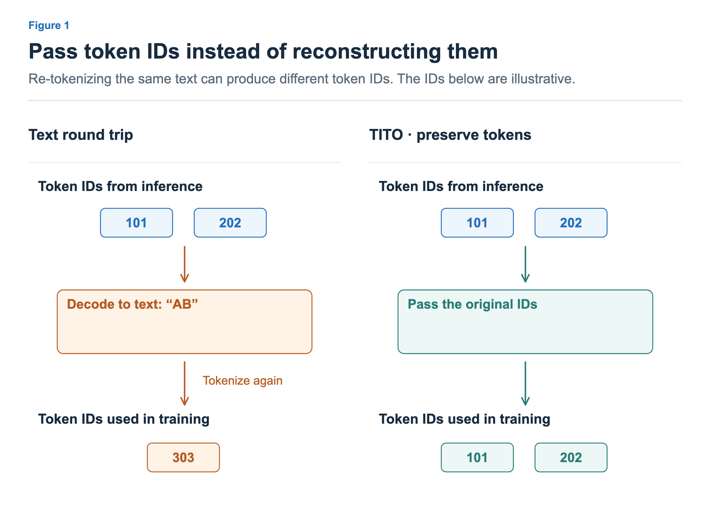
Converting a response to text and tokenizing it again can produce different token IDs. TITO avoids this difference by passing the generated token IDs directly.

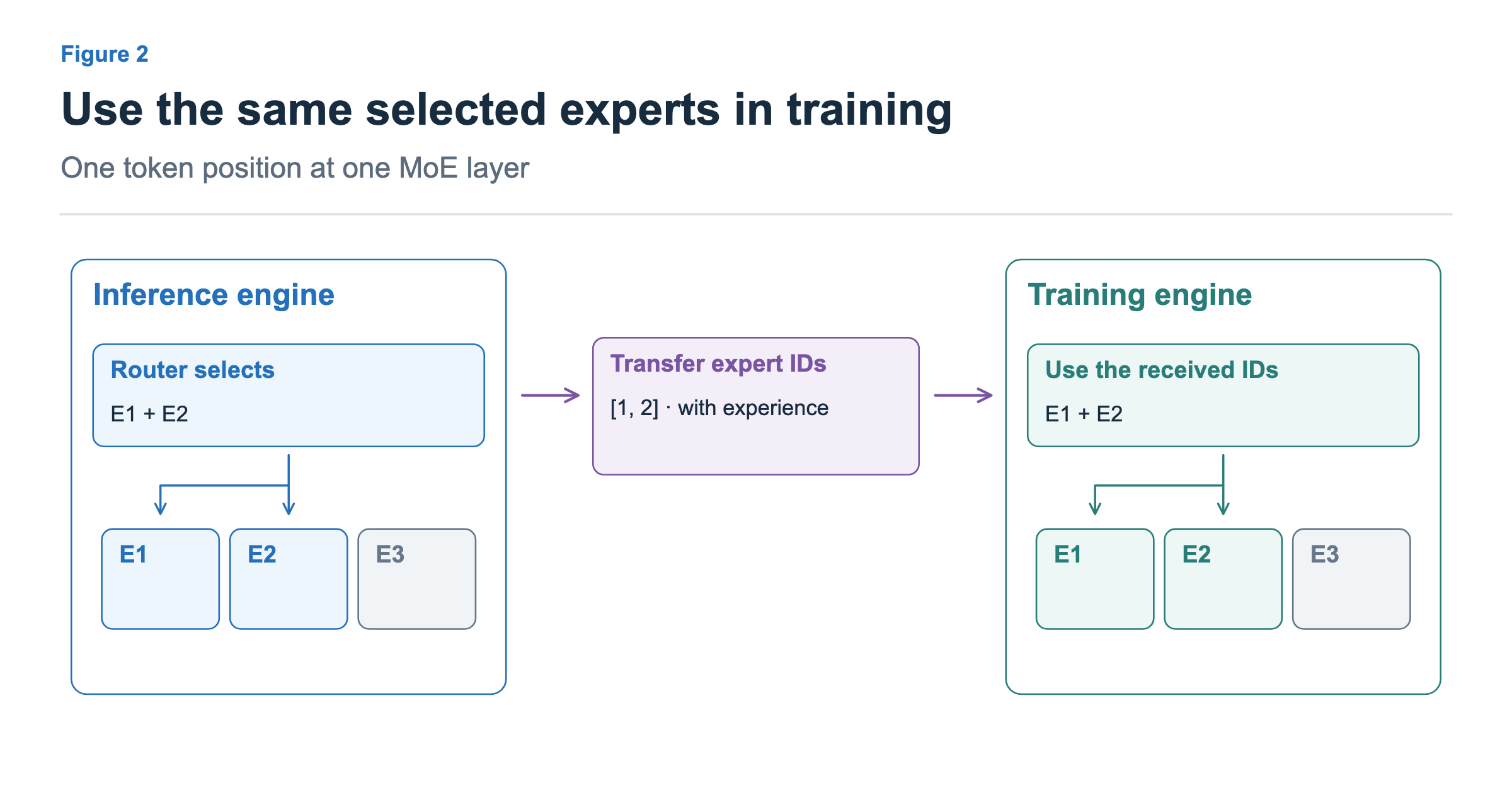
The text round trip turns generated IDs 101,202 into AB and then ID 303. TITO passes 101,202 unchanged to training. The IDs are illustrative.

In an MoE, selecting different experts changes the computation path even for the same token. R3 records the expert IDs selected during generation and reuses them during training. The experts use the current training weights.

The inference router selects E1 and E2. IDs 1,2 travel with the experience to training, which also executes E1 and E2. E3 is not selected.

Quantization changes both cost and computational agreement

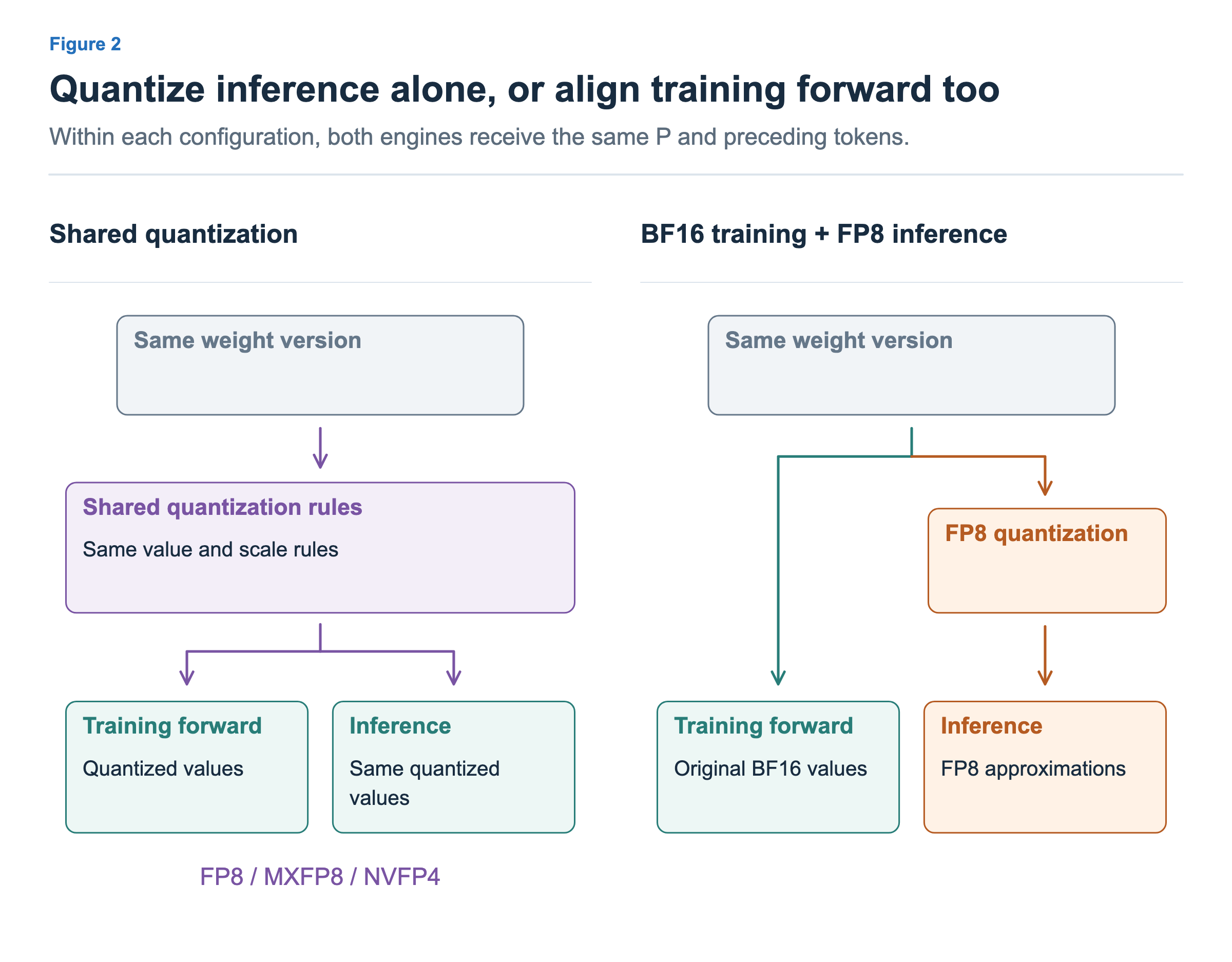
The left configuration applies shared quantization rules so training forward and inference use the same quantized values. The right configuration uses BF16 values in training forward and quantizes only inference to FP8.

We can apply the same quantization convention to both forward passes, or retain BF16 training while running inference in FP8. The latter reduces inference cost but leaves a computational difference. Miles v0.1’s NVFP4 path aligns the training forward pass with the same quantization; it should not be described as a combination with BF16 training.

Article 7: TITO and R3 · Article 8: Quantization configurations

Correct remaining differences with probability ratios

Even with the same weights, differences in operation order, kernels, and precision can change the computed result. Weight updates during learning add another source of difference.

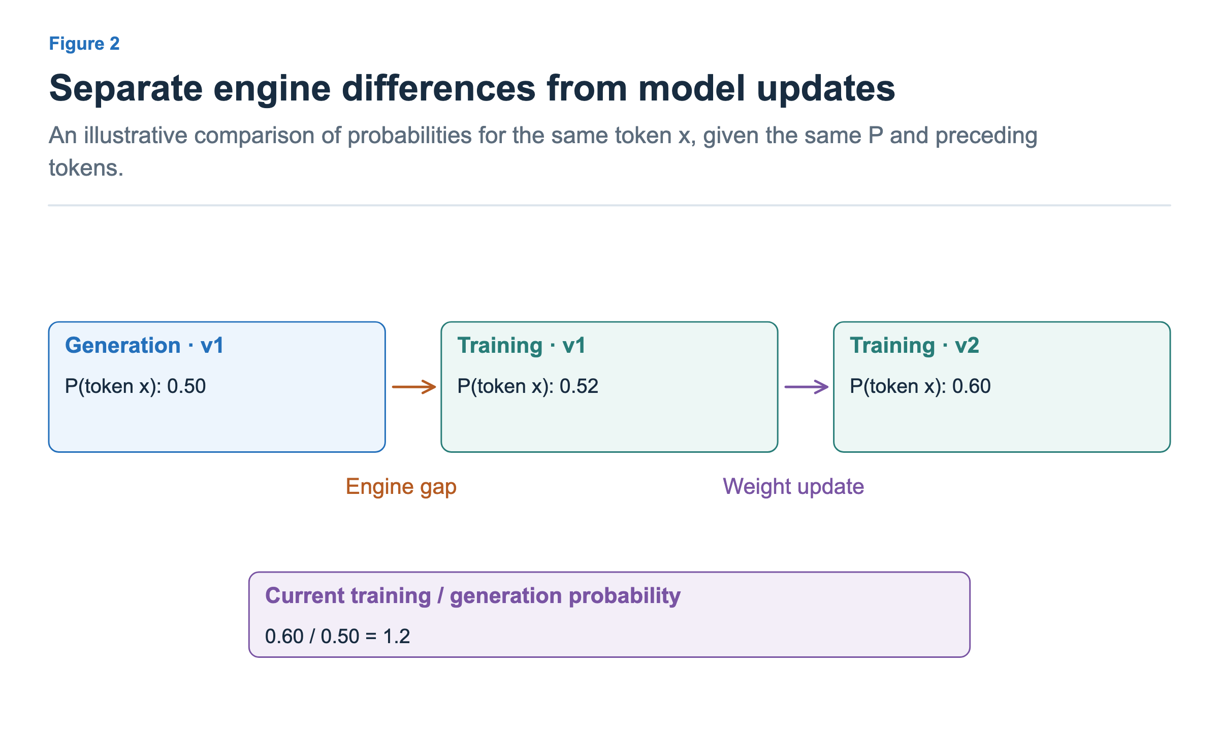
The same token has probability 0.50 in generation engine v1, 0.52 in training engine v1, and 0.60 in training engine v2. The first difference comes from the engines; the second comes from a weight update. Dividing the current training probability by the generation probability gives 1.2.

In the figure, 0.50 → 0.52 is an engine difference, while 0.52 → 0.60 is a model-update difference. The ratio of the current probability to the actual generation probability is 0.60/0.50 = 1.2. This ratio adjusts the weight of the observed choice in learning. Correction does not make the two engines compute identically; clipping or limiting weights is a separate choice for controlling unstable updates.

Article 9: Engine differences and probability correction

Overlapping generation and training can make experience stale

Waiting for all generation to finish before training leaves intervals when one side’s resources are idle. Asynchronous execution generates the next experience while learning from experience that is ready.

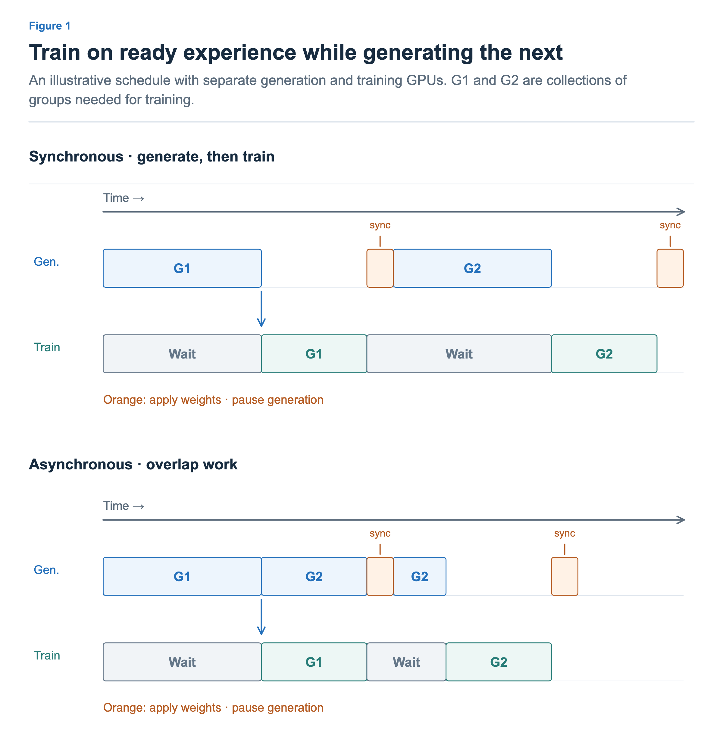
Synchronous execution finishes G1 generation, G1 training, and synchronization before generating G2. Asynchronous execution generates G2 while training on G1, briefly pausing generation for synchronization. Training still waits when data is not ready.

Training weights change at each optimizer update, but the inference engine’s deployed version changes when weight synchronization takes effect. The staleness convention discussed for Miles compares the deployed version with the experience’s generation version. It is not automatically the number of training steps.

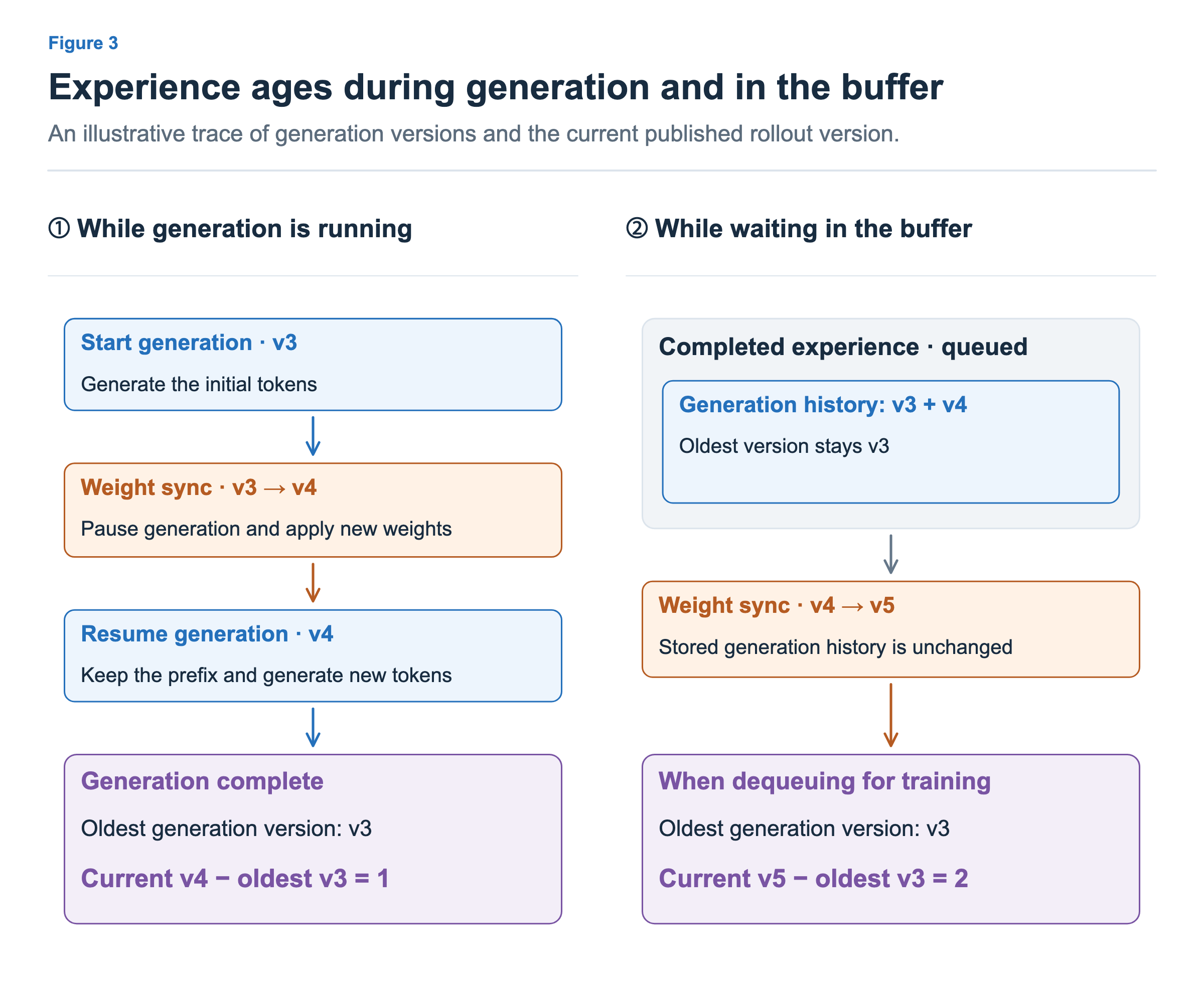
One experience starts with v3 and continues with v4 after synchronization. At completion, the gap between the oldest generation version v3 and current v4 is one. If v5 is published during buffer waiting, the gap becomes two at dequeue.

Experience can become stale during a long generation run or while waiting in the buffer after completion. The figure illustrates a configuration that can continue generation after an intermediate synchronization. We must consider both the benefit of reduced waiting and the cost of correcting or discarding stale experience.

Article 10: Asynchronous execution and staleness

Inference optimization extends to the whole agent execution

Reuse computation while accounting for queueing

Reusing a shared prefix’s KV cache can reduce input computation. But if the engine holding that cache has a long queue, another engine may finish sooner.

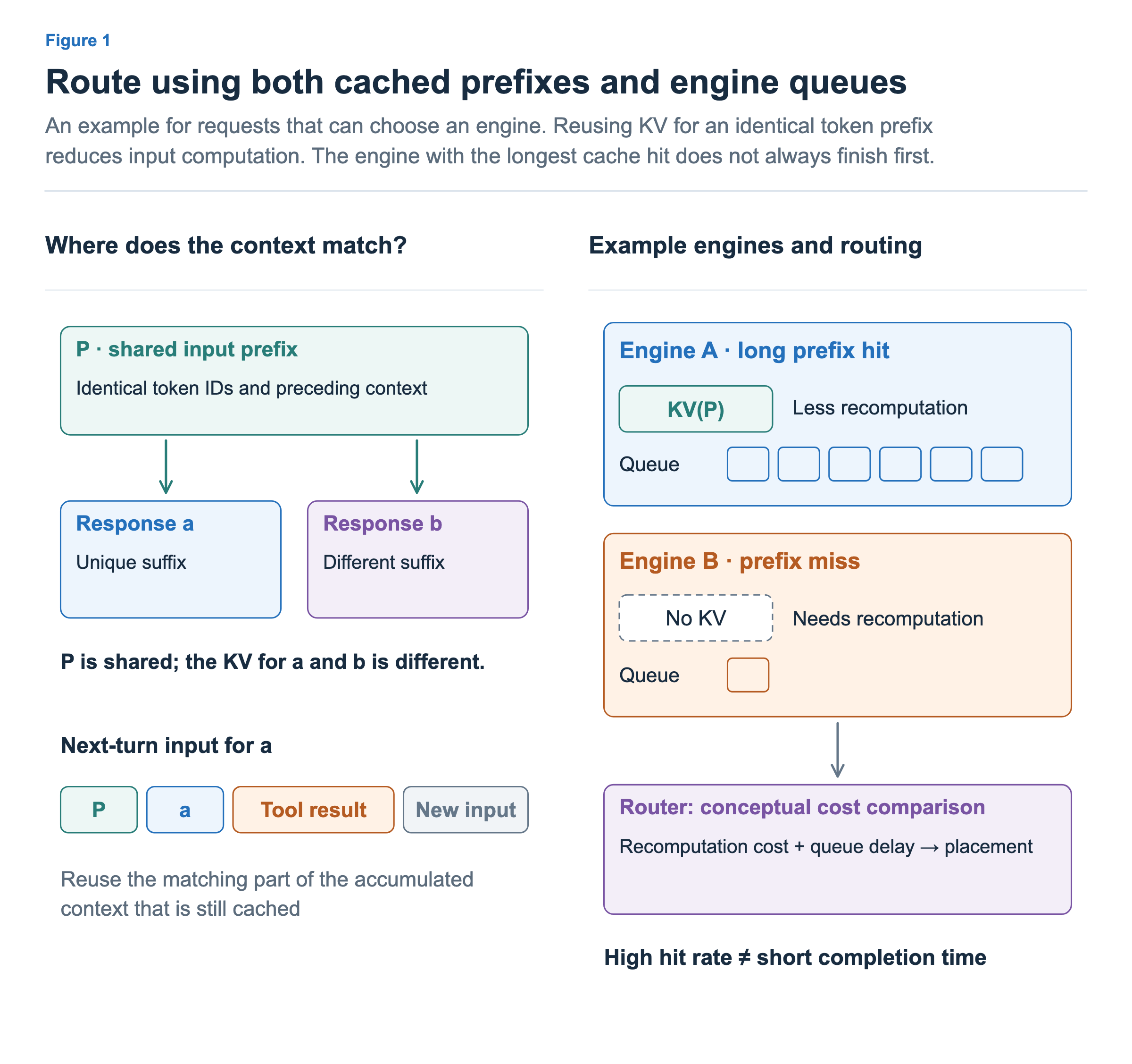
Responses a and b branch from a shared input P; what can be shared is the KV cache of the matching prefix P. Engine A has P cached but a long queue, while engine B lacks the cache but has a short queue. The router considers both recomputation cost and waiting.

Inference optimization also includes filling vacant batch slots, speculative decoding that verifies multiple candidate tokens together, and generating candidates with MTP. These approaches target repeated computation, unused capacity, and the cost of sequential generation, respectively.

The task continues after a model call ends

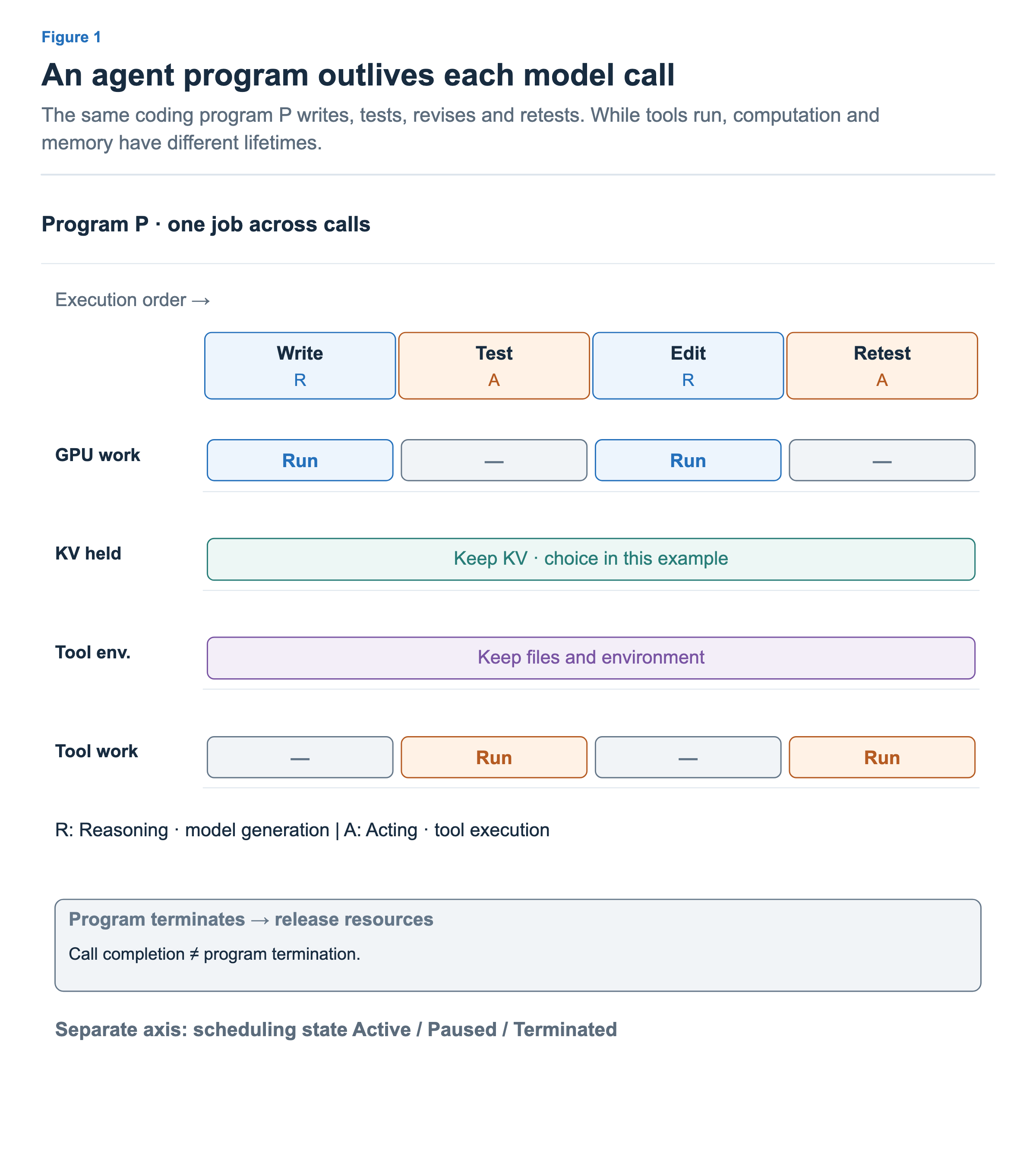
Program P proceeds through code writing and editing as Reasoning, and testing and retesting as Acting. GPU computation and tool execution occur in different intervals; in this example, KV, files, and the execution environment persist between calls. Resources are reclaimed when the task ends.

While an agent waits for a tool result, GPU computation can stop while KV and the tool environment remain allocated. ThunderAgent uses program state to decide execution, pausing, and restoration. On a separate CPU tool server, environment preparation, execution queues, and resource reclamation also affect completion time. The scope of optimization expands from token generation to the lifetime of the whole task.

Article 11: Inference optimization · Article 12: Scheduling the whole agent

Resuming generation with new weights continues the loop

The final step is weight synchronization. Prepare weights in the partitions and format required by inference, transfer them over a path suited to the communication environment, and resume once the new policy is ready to use.

Broadcast is a baseline path over a shared GPU communication fabric; P2P exploits parallel transfers across nodes; disk-delta uses shared storage. Choosing a suitable method requires comparing conversion, transfer, and application costs together.

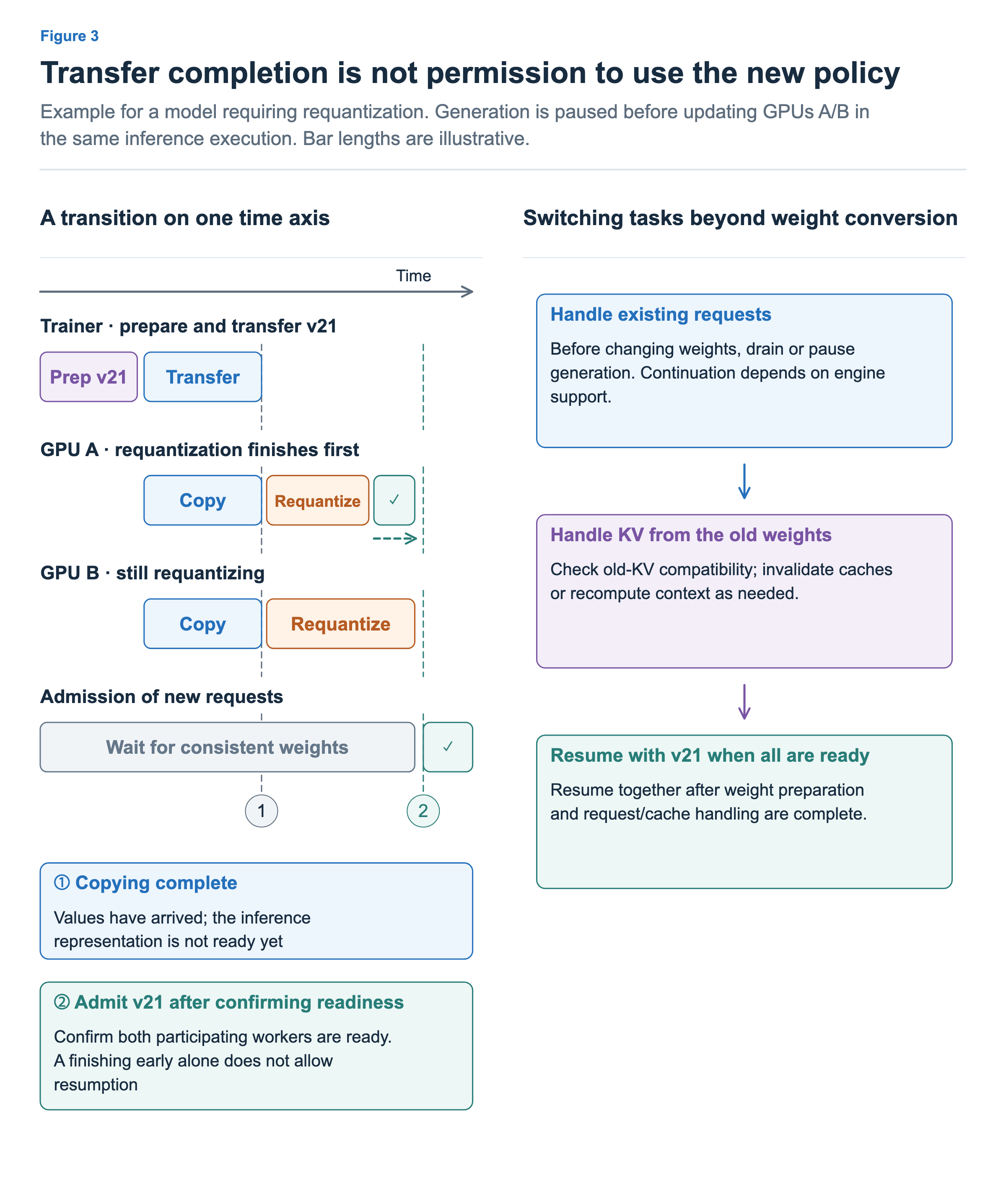
The trainer prepares v21 and transfers it to A and B. After copying finishes, each GPU still has requantization to perform; A becomes ready first and B later. New v21 requests are allowed after both participating workers are confirmed ready. Rules for handling existing requests and old KV are determined before the transition.

For models requiring requantization, as in the figure, conversion must still finish after copying completes. The participating inference GPUs must be ready, and existing requests and KV must be handled, before generation can proceed with a consistent new policy.

Token choice → evaluation and learning signals → loss and weight updates → new-weight transfer → the next token choice. The learning principles in the first half and the systems in the second half together complete this one loop.

Article 13: Preparing, transferring, and resuming with new weights