DeepSeek's KV Cache: From 3.9 MB to 890 B per Token

One of the main costs of long-context inference is the KV cache: the Keys and Values of earlier positions, stored so they do not have to be recomputed every time a new token is generated. As the KV cache article showed, this storage grows in proportion to context length and is multiplied by the number of requests served at once. So how much the cache grows when the context gains one token goes a long way toward setting the cost of long-context inference.

DeepSeek changed its attention design several times between V2 and V4.1. This article follows those changes through one number, the KV cache per token. A hypothetical MHA model with V2’s dimensions, storing every head’s Key and Value, would use about 3.9 MB per token. V4.1-Flash uses 890 B per token (the growth per token in a long context; the local KV that keeps recent positions is separate), about 1/4,400 of that.

This reduction did not happen in a single step. The cache per token can be seen roughly as built from four factors.

KV cache per token ≈ width of the stored vector (dimensions)
                     × number of layers storing KV
                     × bytes per element
                     ÷ compression ratio (how many tokens' KV is merged into one)

V2’s MLA narrowed the width of the stored vector. V3.2’s DSA reduced the number of positions read, rather than the amount stored. V4’s CSA and HCA use compression along tokens, merging the KV of several tokens into one stored vector, and V4.1’s CSA2 lets layers share KV to reduce the number of layers that store KV for the whole context. Along the way, bytes per element also dropped from BF16 (2 B) to FP8 (1 B) and then FP4 (0.5 B). Below, we look at what changed in each generation through figures and then work out the numbers ourselves.

KV cache per token at a glance

First, here are the numbers for five models in one figure. All bars use a log scale. Each step is 10×, so differences in bar length should not be read as ratios. Read the number at the end of each bar together with “≈1/N of MHA”.

Figure 1 · KV cache: what is stored and what is readBoth in deployed cache formats · left: storage added per token · right: reads per generated token (128K context)Two graphs compare a hypothetical MHA, V2, V3.2, V4-Flash and V4.1-Flash. Left: KV cache added per token in a long context, from 3,932,160 B to 890 B. Right: bytes read across all layers to generate one token in a 131,072-token context, from 515 GB to 35.0 MB, with search keys dominating from V3.2 on. The graphs use different units and scales.

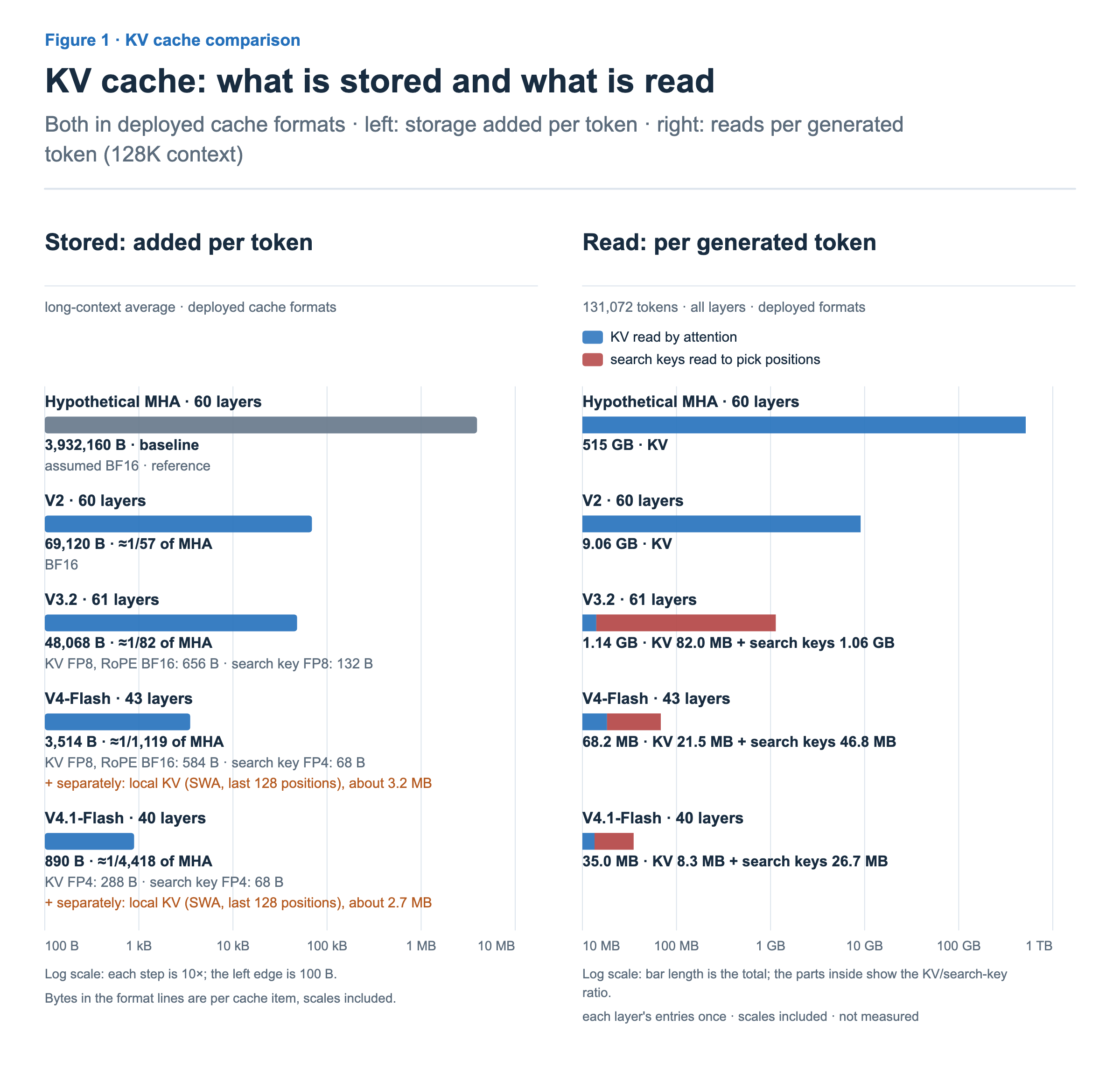
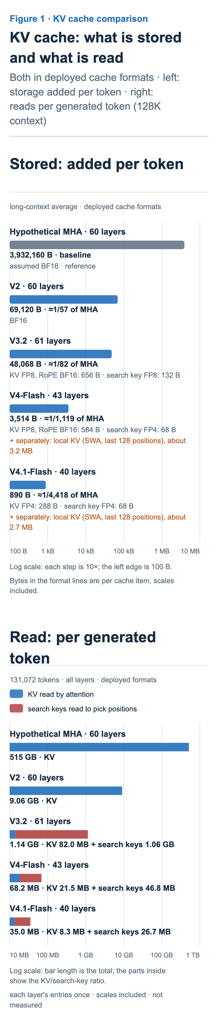
Storage. The amount added per token in a long context, computed in the deployed cache formats this article adopts. A deployed cache format is how a real serving engine stores the cache (its precision and scale layout). V2 is BF16, V3.2 and V4 mix FP8 and BF16 in their KV, and V4.1 stores global KV (the KV that builds up over the whole context) in FP4. The hypothetical MHA is a reference that assumes BF16 storage. This section focuses on this panel.

Reads. What all layers read to generate one token in a 128K context, computed in the same deployed cache formats as the left panel. Bar length (the total) is on a log scale, but the colored parts inside a bar split it by the ratio of KV to search keys. The units differ, so this panel has its own scale; it is covered in detail in the V3.2 section.

The format and bytes are listed under each bar. The bytes in a format line are the size of one item stored in one layer; the bold number combines them over the layers and the compression ratio into a per-token value. The section on each version shows how this is calculated. The scale in a format line is a factor that brings values stored at low precision back to their original size.

A few things stand out. On the storage side, V3.2 is smaller than V2, but only because it stores in FP8. At the same precision, V3.2 is actually larger, because it also stores the search keys used to pick positions. V4 drops by more than an order of magnitude, and V4.1 reaches 890 B. Under V4 and V4.1, an orange line adds a local KV (SWA) that is kept separately: the KV of only the last 128 positions. By the end of this article, you will see why these values come out the way they do.

The baseline: MHA that stores every head’s Key and Value

The starting point is core attention. In MHA, each layer builds a Key and a Value for every head and stores both in the cache. Plugging in V2’s numbers, storing one token takes:

Hypothetical MHA: 60 layers × 128 heads × (Key 128 + Value 128) × 2 B (BF16)
                = 3,932,160 B ≈ 3.9 MB

At about 3.9 MB per token, a 128K-token context (131,072 positions) needs about 515 GB of cache for a single request. In decode, this whole cache is read for every new token. Storage and reads are both a problem. MQA and GQA cut this value by letting several heads share Key and Value. DeepSeek took a different path.

DeepSeek-V2

V2 narrows the width of the stored vector with MLA (Multi-head Latent Attention). Instead of per-head Key and Value, it stores a small shared vector (the latent) from which they can be built, plus a positional Key. The model does not compress MHA’s Key and Value and restore them; it is trained from the start with Key and Value built from the latent. Below we look at what is stored, how attention is computed without expanding per-head Key and Value (rebuilding them from the cache), and then the storage per token. Figure 2 shows the effect.

Figure 2 · KV cache stored and read: V2Storage and reads of MHA and V2The two graphs of the first figure up to V2, with the V2 row highlighted.

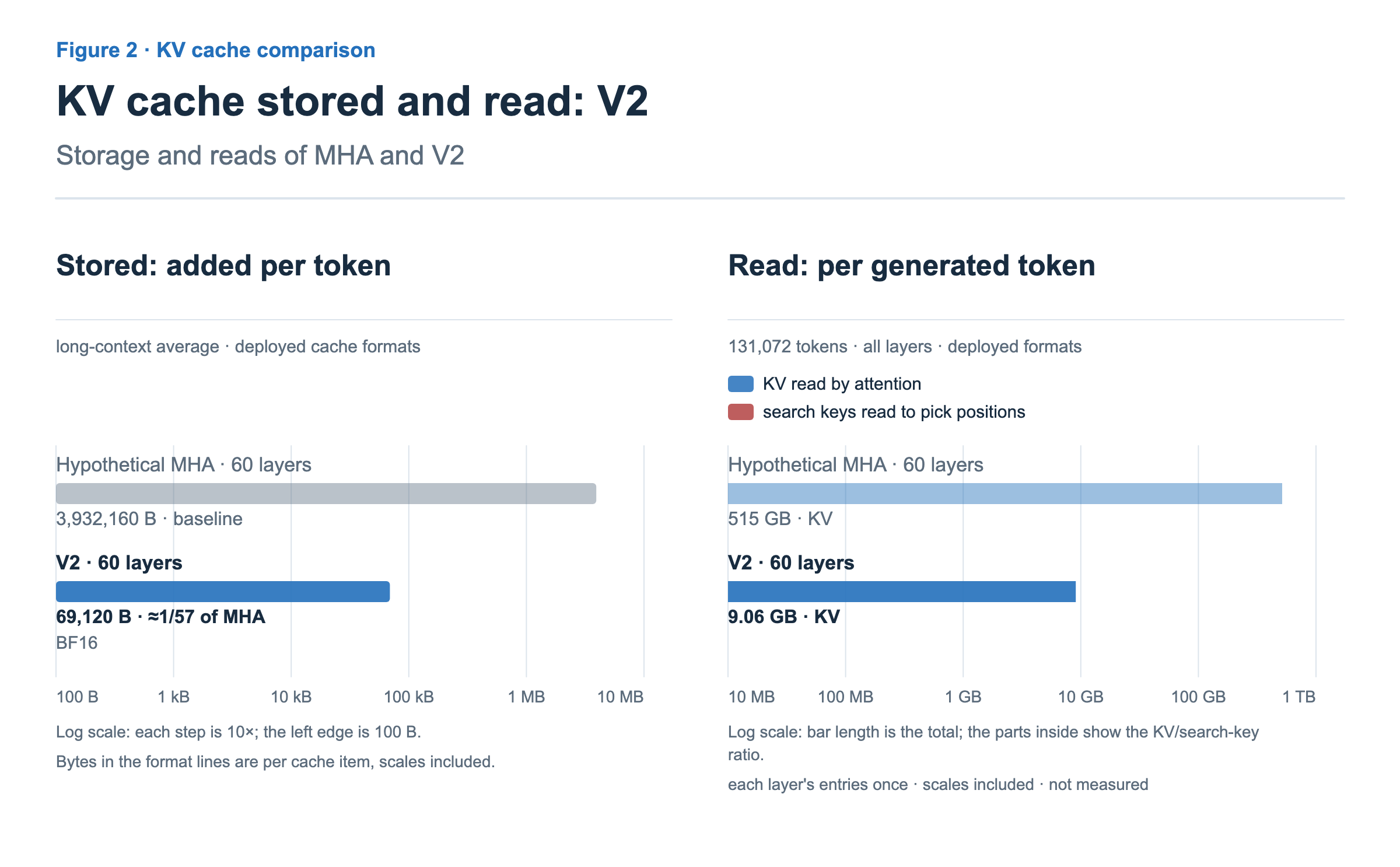
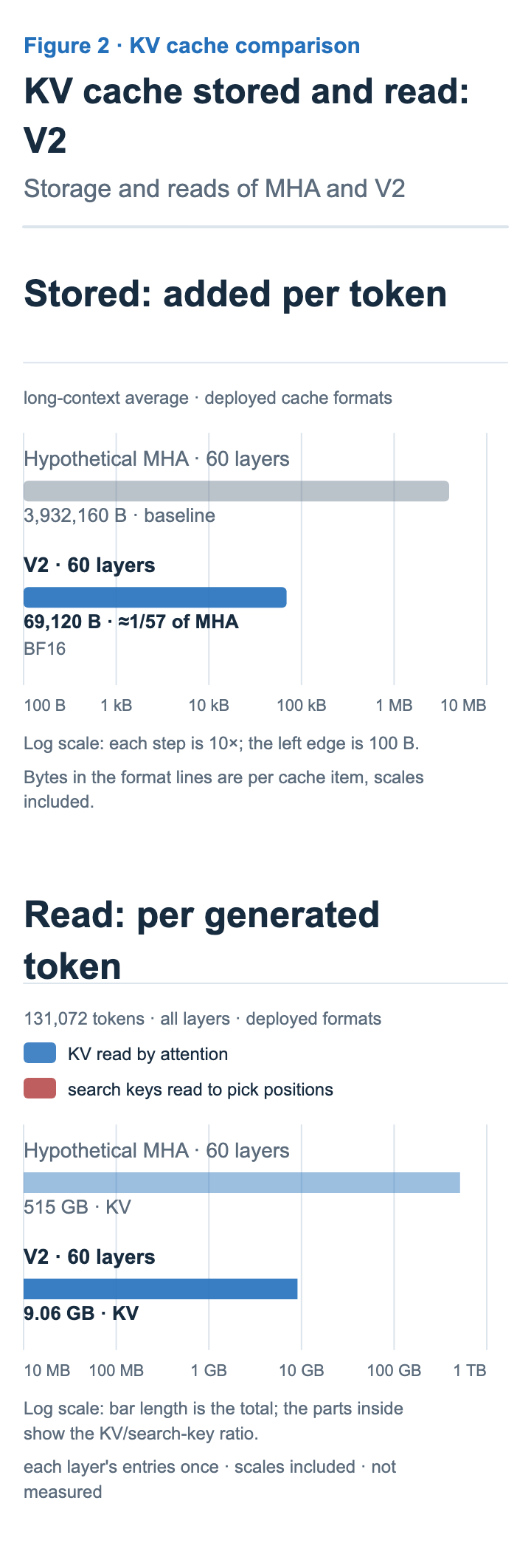
V2 uses 69,120 B per token, about 1/57 of MHA.

At a context of 131,072 tokens, the reads to generate one token drop from about 515 GB for the hypothetical MHA to about 9.06 GB. Both models store in BF16.

MLA: three paths from the same input

Before the figures, a word on notation. In this article’s matrix figures, activations have tokens as rows and features as columns, and weights have the shape [input, output]. Box widths show only the order of column sizes and are not to scale. Purple boxes are learned weights W, and the superscript of W says what the weight does.

The figures draw all T tokens of the context computed at once. When decode produces one new token, the Query side is only the last row, while the Key and Value side is all T cached positions.

Figure 3 shows how the input X branches into three paths within an MLA layer: one for the queries, one for the shared KV latent, and one for the positional key. Each path is drawn starting again from the same input X.

Figure 3 · MLA branches from one inputThree paths from X: the query, the shared KV latent, the rotary keyShared X is projected to a query latent, a KV latent and a rotary key. Each latent feeds two weights. Box widths follow the order of column sizes. Cᴷⱽ and Kᴿ are cached, and every head shares Kᴿ.

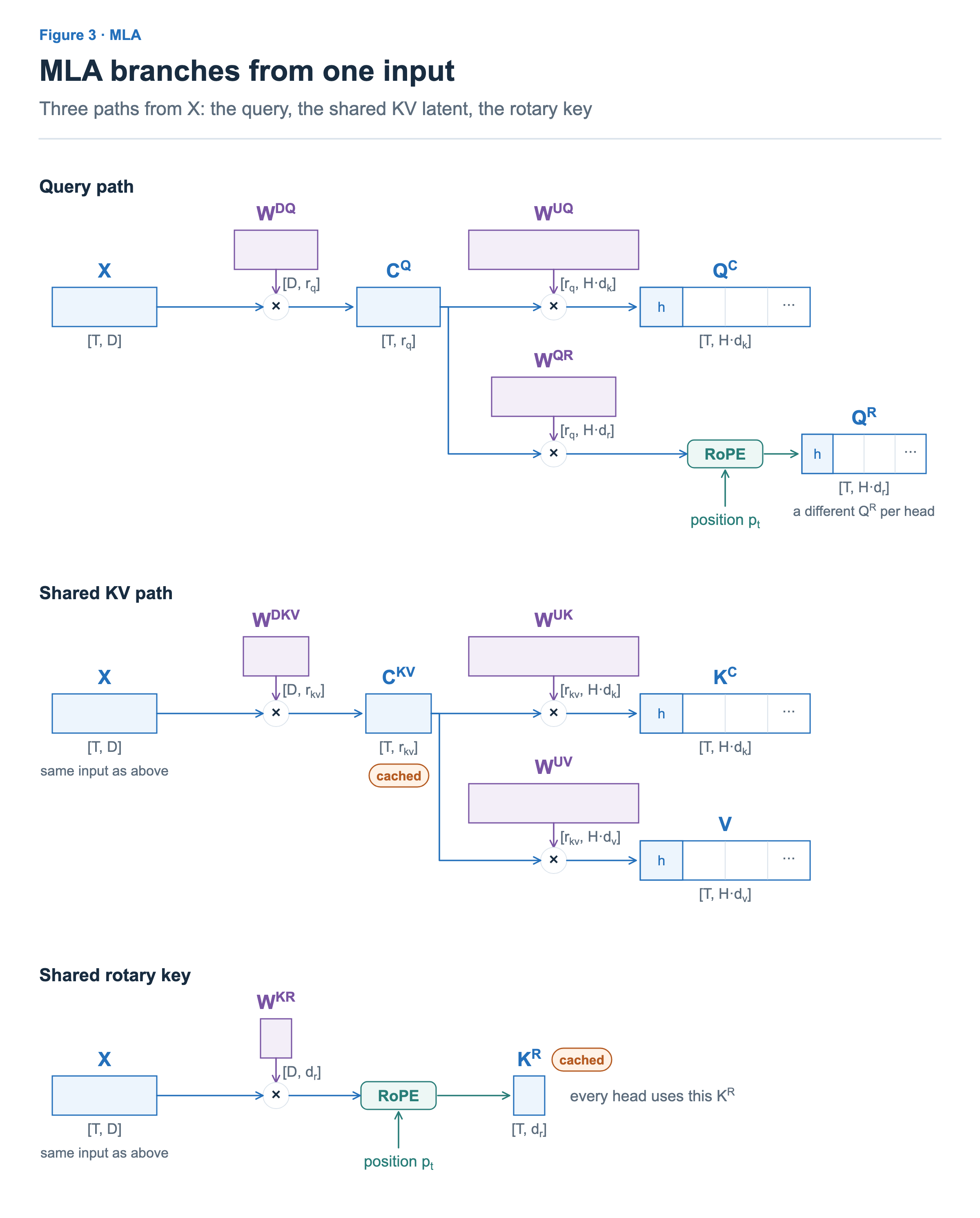
Query path. X is reduced to a Query latent C^Q (1,536 dimensions), and from it each head builds a content query Q^C_h and a positional query Q^R_h. Queries are not stored in the KV cache for later tokens.

Shared KV path. X is reduced to the 512-dimensional C^KV, which is stored in the cache. Per-head Keys and Values are not stored, because they can be built by multiplying C^KV by per-head weights W^UK_h and W^UV_h.

Shared rotary key. One 64-dimensional K^R with RoPE applied is shared by all heads and stored in the cache. Position information goes only into this K^R; C^KV gets no RoPE. Why the positional part is kept separate has to do with “absorption,” so it is explained after absorption.

What stays in the cache is C^KV (512 dimensions) and K^R (64 dimensions).

Content score and positional score

Figure 4 splits the attention computation of one head into two lines. The top line goes from scores to probabilities; the bottom line uses the probabilities to weight the Values and produce the output.

Figure 4 · Add two scores for attentionOne head h · content score + rotary scoreFor head h, multiply content parts and rotary parts separately and add the two scores, which equals the dot product of the concatenated Q and K. After scaling, causal masking and softmax, the probabilities weight V. All head outputs are concatenated and projected. Box widths follow the order of column sizes.

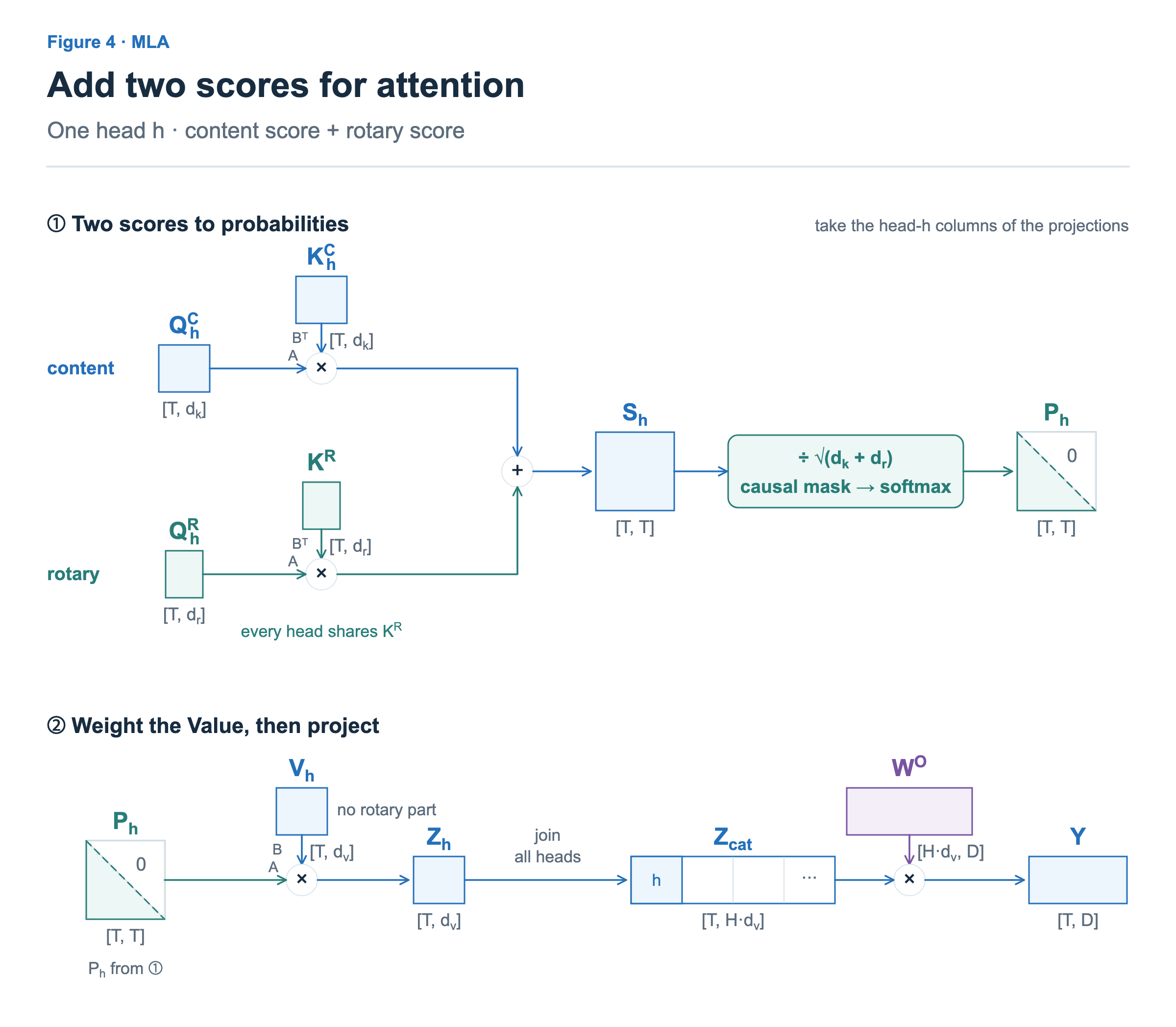
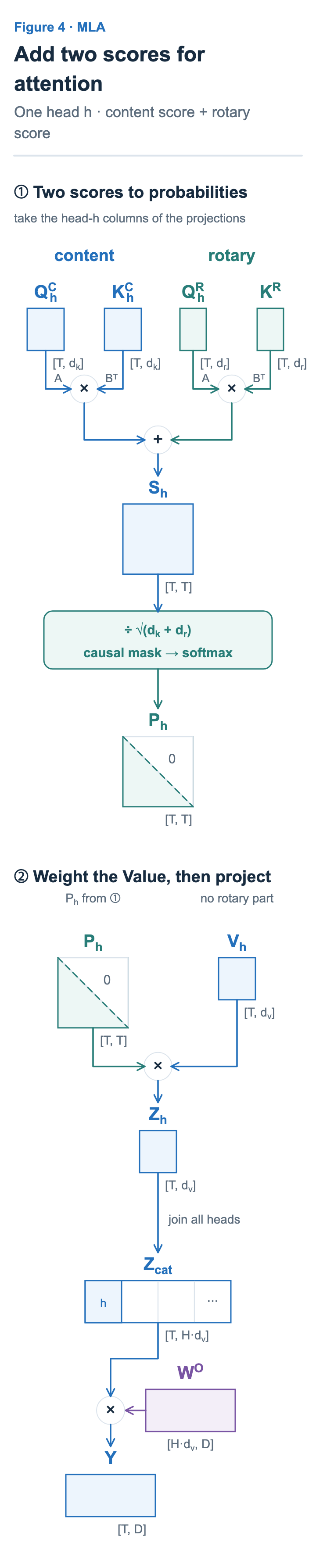
① From scores to probabilities. The score is the sum of two parts: the content score Q^C_h (K^C_h)^T, from multiplying content components, and the positional score Q^R_h (K^R)^T, from multiplying positional components. This equals the dot product of a Query and Key formed by concatenating the two components. Dividing the summed score S_h by √(d_k + d_r) and applying the causal mask and softmax gives the probabilities P_h.

② On to the output. The probabilities P_h weight V_h to give Z_h; the results of all heads are concatenated and projected by W^O.

From this figure alone, MLA looks as if it still expands every head’s Key and Value for the computation. Then storage would be small, but each step would need computation to rebuild Key and Value. Decode avoids this rebuilding with absorption, which changes the order of the multiplications.

Computing without expanding Key and Value

Figure 5 computes the same content score in three ways. The three lines are not steps run one after another; they are three orders of computation that give the same result from the same C^Q and C^KV.

Figure 5 · The same score without expanding the KeyContent score of one head · three orders, one resultAll three views start from C^Q and Cᴷⱽ. Moving the key expansion weight to the query side gives the same content score without expanding K. The two query-side weights can also be merged in advance.

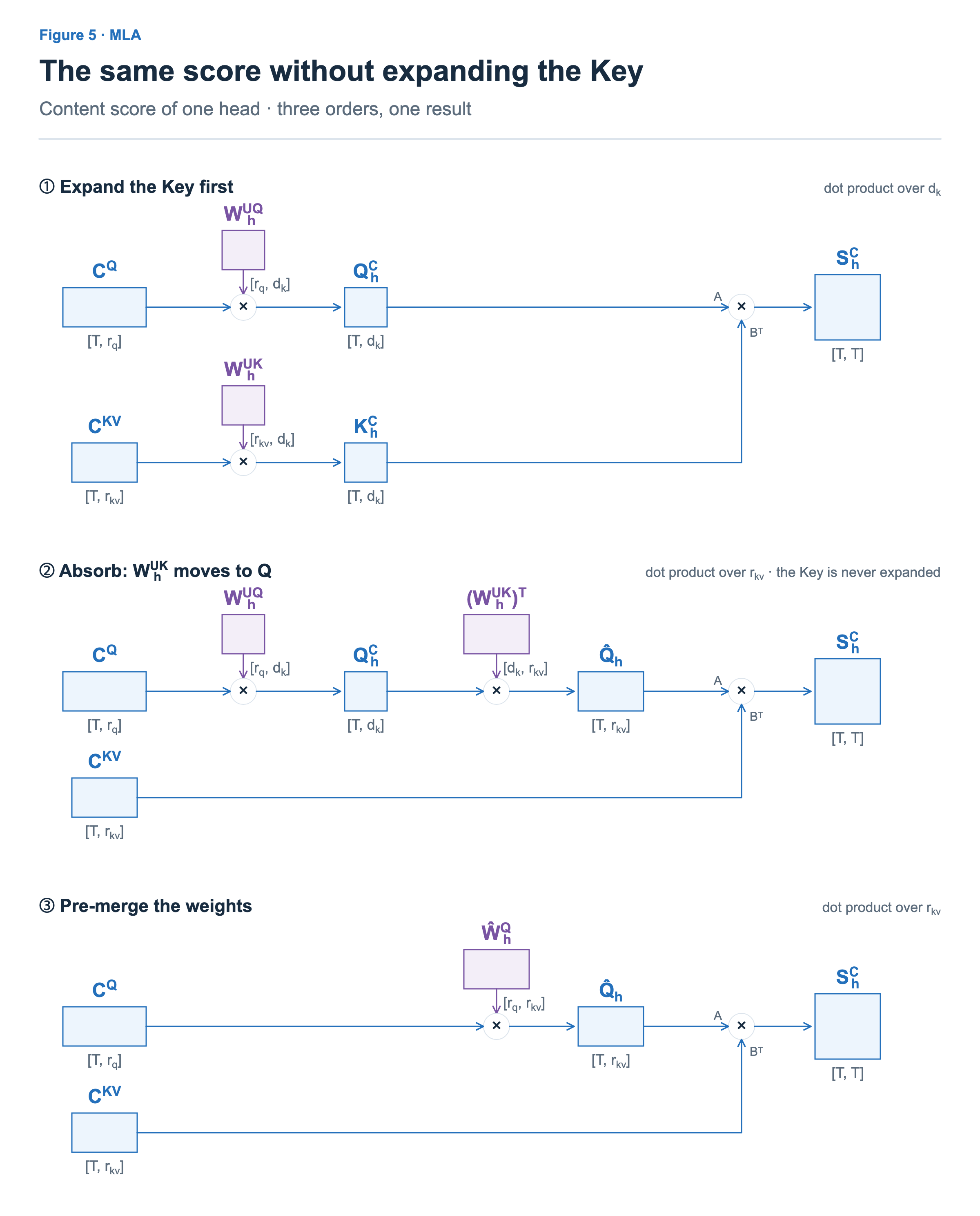
① Expand. As in Figure 4, build the per-head K^C_h, then multiply by the Query. The dot product runs over d_k dimensions.

② Absorb. Only the parentheses move. By associativity of matrix multiplication, Q^C_h (C^KV W^UK_h)^T = (Q^C_h (W^UK_h)^T) (C^KV)^T. Multiplying W^UK_h on the Query side first gives a 512-dimensional Q̂_h, which is multiplied directly with C^KV from the cache. K is never expanded.

③ Pre-merge the weights. The two Query-side weights are merged into one in advance: Ŵ^Q_h = W^UQ_h (W^UK_h)^T. This is mathematically the same, but the merged weight can be larger, so real implementations do not necessarily use it.

The three forms produce algebraically the same content score. With finite precision and quantization, rounding error can differ slightly. All three only change the order in which the content score is computed; the positional score Q^R_h (K^R)^T and the scaling by √(d_k + d_r) (a divisor of the score, unlike the scales stored with quantized values) stay as they are.

With absorption, the dot product at each position runs over r_kv (512) instead of d_k (128), four times longer. In exchange, multiplying every cached position by W^UK_h to expand the Key (a 512×128 product per position) and reading that expanded Key both disappear; the Query side multiplies by W^UK_h just once. In decode, with a single Query, this difference is large and absorption wins. In prefill, with many Queries, a Key expanded once is shared by all of them, so computing with the expanded Key can be better.

Why the positional part is kept separate. Absorption builds one Q̂_h and multiplies it with C^KV at every position, so nothing between the Query and C^KV may change from position to position. If RoPE were applied to the content Key built from C^KV, then in the figures’ row-vector notation the score at position s would take the form q R(t − s) (W^UK_h)^T c_s^T (c_s is C^KV at position s). An R(t − s) that differs by position sits in between, so no single Q̂_h exists. That is why MLA puts position information only into the small K^R with RoPE, and uses absorption only on the content part, which has no RoPE (MLA storage article).

With the score in hand, the same can be done for how the probabilities combine the Values. The three lines of Figure 6 are again three orders of computation with the same result. In Figure 6, W^O_h is the block of rows of Figure 4’s output weight W^O that belongs to head h, and Y_h is head h’s contribution to the final output. Adding Y_h over all heads gives Figure 4’s Y.

Figure 6 · The same output without expanding the ValueSame probabilities P_h · three orders, one resultWeight the latent before expanding V. Merge the value expansion and the per-head output weight to produce the same contribution. Sum the contributions across heads.

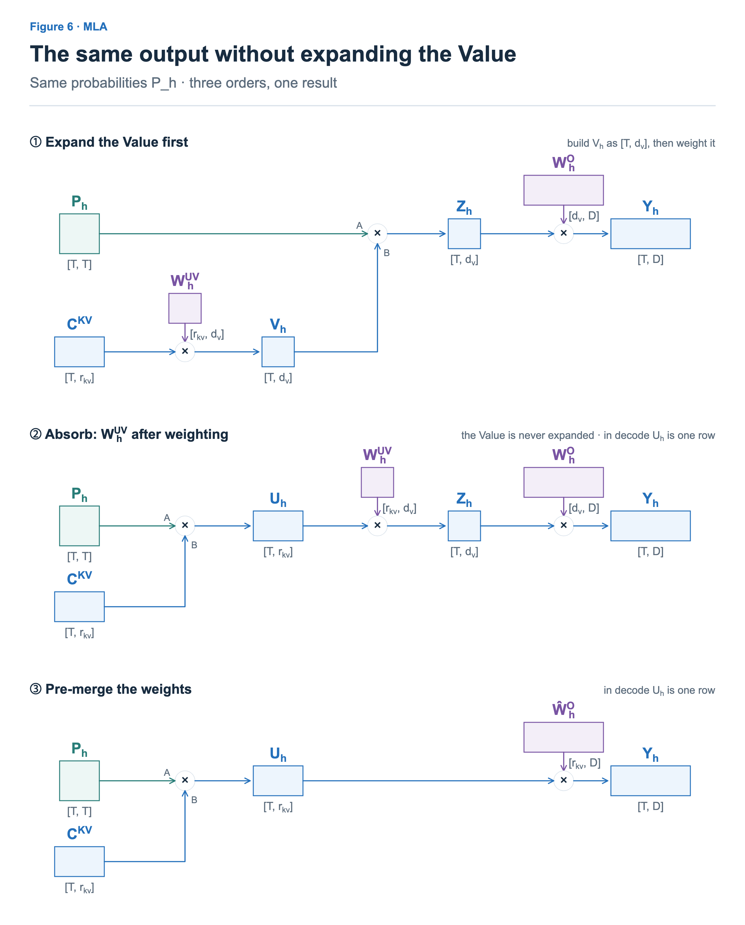
① Expand. Expand V_h to [T, d_v], then take its weighted sum with the probabilities P_h.

② Absorb. First, use the probabilities to take a weighted sum of the rows of C^KV, giving U_h. Then multiply U_h by W^UV_h and the output weight. the Value is never expanded: expanding means building the Value for all T positions, while ② multiplies W^UV_h only into the result after weighting (one row in decode).

③ Pre-merge the weights. W^UV_h and W^O_h are merged into one in advance: Ŵ^O_h = W^UV_h W^O_h.

Swapping the order of the weighted sum and the matrix multiplication gives the same result. This way, a decode step completes its computation while reading only C^KV and K^R from the cache. The derivation of absorption is traced with a small example in the MLA computation article.

Calculating V2’s KV cache

Now V2’s number follows. Each layer stores 512 dimensions of C^KV and 64 of K^R.

V2: 60 layers × (C^KV 512 + K^R 64) × 2 B = 69,120 B  (about 1/57 of MHA)

V3 has the same MLA structure with 61 layers, so 61 × 576 × 2 = 70,272 B. That is why this article does not treat V3 separately.

MLA cut storage sharply, but the range that is read is unchanged. Each decode step still reads C^KV at every earlier position. In a 128K context, V2 reads 60 layers × 131,072 × 1,152 B ≈ 9.06 GB (1,152 B = (C^KV 512 + K^R 64) × 2 B) per step. That is far less than MHA’s 515 GB, but it keeps growing as the context gets longer.

DeepSeek-V3.2

V3.2 keeps MLA and adds DSA (DeepSeek Sparse Attention) to choose which positions to read. A small lightning indexer scores positions and picks up to 2,048 of them, and the main attention uses only the picked positions. According to the report, the indexer is trained to follow the probability distribution the main attention actually produces. Below we look at how the search key is built, the score that picks positions, and the main attention over the picked positions, and then work out storage and reads. Figure 7 shows the effect.

Figure 7 · KV cache stored and read: V3.2MHA to V3.2 · DSA cuts the positions read (at equal precision, storage grows)The two graphs of the first figure up to V3.2, with the V3.2 row highlighted.

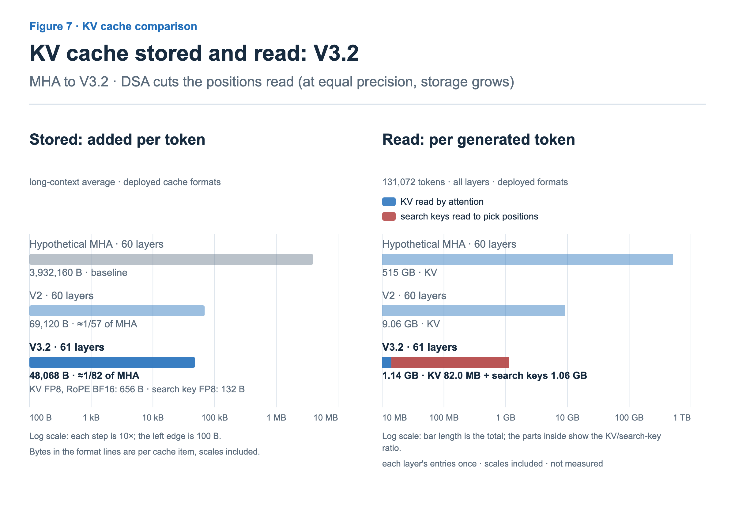
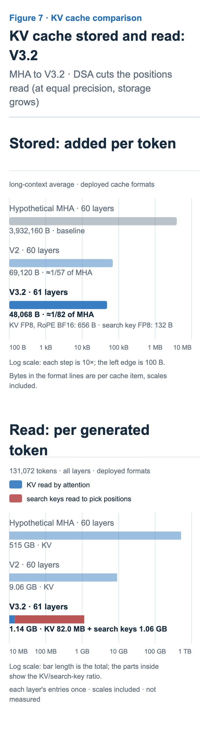
V3.2 uses 48,068 B per token. It is smaller than V2 because of a deployed format that uses FP8. If every value were stored in BF16, the added search key would actually make it larger.

With position selection and lower-precision storage together, reads drop to about 1.14 GB, about 1/8 of V2. Most of it is search keys.

DSA: three things the indexer builds

The indexer is a small module that picks the positions to read in a way similar to the scoring part of attention. It does not weight Values into an output. Values on the indexer side carry the superscript I (indexer): q^I_j is the query of indexer head j, k^I is the search key, w^I is the head weight, and the weights that produce them are W^IQ, W^IK, and W^Iw. The subscript j numbers indexer heads, which are separate from the main attention’s heads h. As Figure 8 shows, the indexer builds three things.

Figure 8 · Three things the indexer buildsFrom MLA’s query latent and X · query, key, head weightsThe lightning indexer builds per-head queries from MLA’s query latent Cᵠ, and from X a key shared by all indexer heads plus one weight per head. The indexer key is cached in FP8. Box widths follow the order of column sizes.

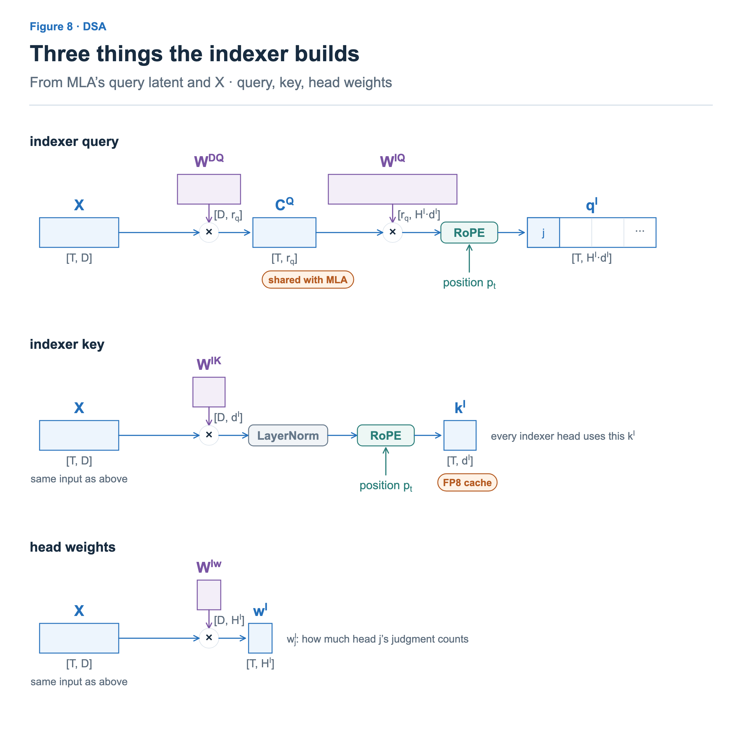
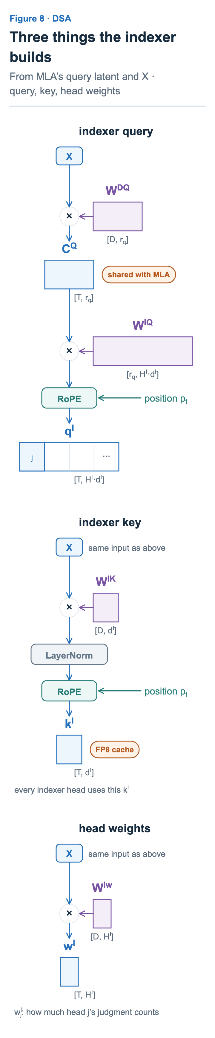
Indexer query. q^I_j is built for each head j from MLA’s Query latent C^Q (number of indexer heads H^I = 64, width per head d^I = 128). It reuses the same latent as the main attention.

Search key (labeled indexer key). Only one k^I is built from the input X and shared by all indexer heads. This value builds up in the cache, because later tokens need k^I at each earlier position to evaluate it. The RoPE in the figure applies to 64 of the 128 dimensions, and LayerNorm is a normalization that sets a vector’s mean and variance. Compared at the same precision, this extra key increases storage.

Head weights. w^I is built from X and sets, for each token, how much each of the 64 heads’ judgments counts.

The score that picks positions

The indexer combines its query, key, and head weights to rank the positions each query may read. Figure 9 draws the scores of all queries as one [T, T] matrix: rows are queries and columns are candidate positions. ⊙ is an element-wise product; the head weight w^I_j has one value per query row, so that value multiplies every candidate score in the row.

Figure 9 · A score that picks which tokens to readScore of indexer head j → sum over indexer heads → top-k per rowFor each indexer head j, the query is dotted with the shared key, passed through ReLU and scaled by the head weight. Summing over heads gives the score I; each row keeps its top-k positions as the selection mask M.

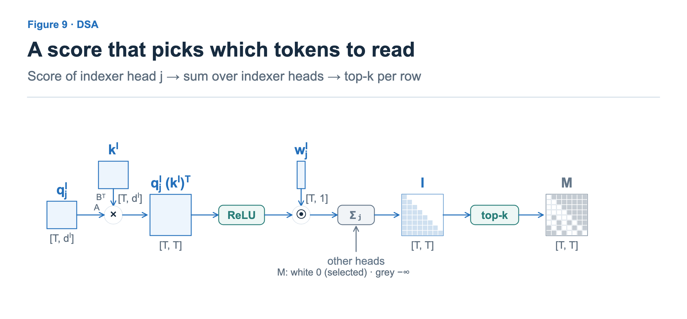
For each head, take the dot product of the query and the shared key, apply ReLU (which turns negatives into 0), and multiply the result by the head weight. Then sum over all heads.

From the score I, each row picks up to 2,048 highest-scoring positions among the positions that query can see (itself included), giving a selection mask M: 0 for picked positions and −∞ for the rest.

In the report’s notation:

I(t, s) = Σⱼ w^I(t, j) × ReLU( q^I(t, j) · k^I(s) )

The indexer has no softmax, and w^I is not a probability. The score is used only for ranking.

MLA that reads only the picked positions

Once the selection is set, the main attention keeps probability only at those positions. Figure 10 is ② of Figure 5, absorbed MLA, with the selection mask M added.

Figure 10 · MLA that keeps probability only at picked positionsAbsorbed MLA scores + selection mask M · one headAdd the indexer’s selection mask M to the absorbed MLA score S_h, the sum of content and rotary scores, then apply softmax. P_h is nonzero only at the selected positions per row and weights Cᴷⱽ into U_h.

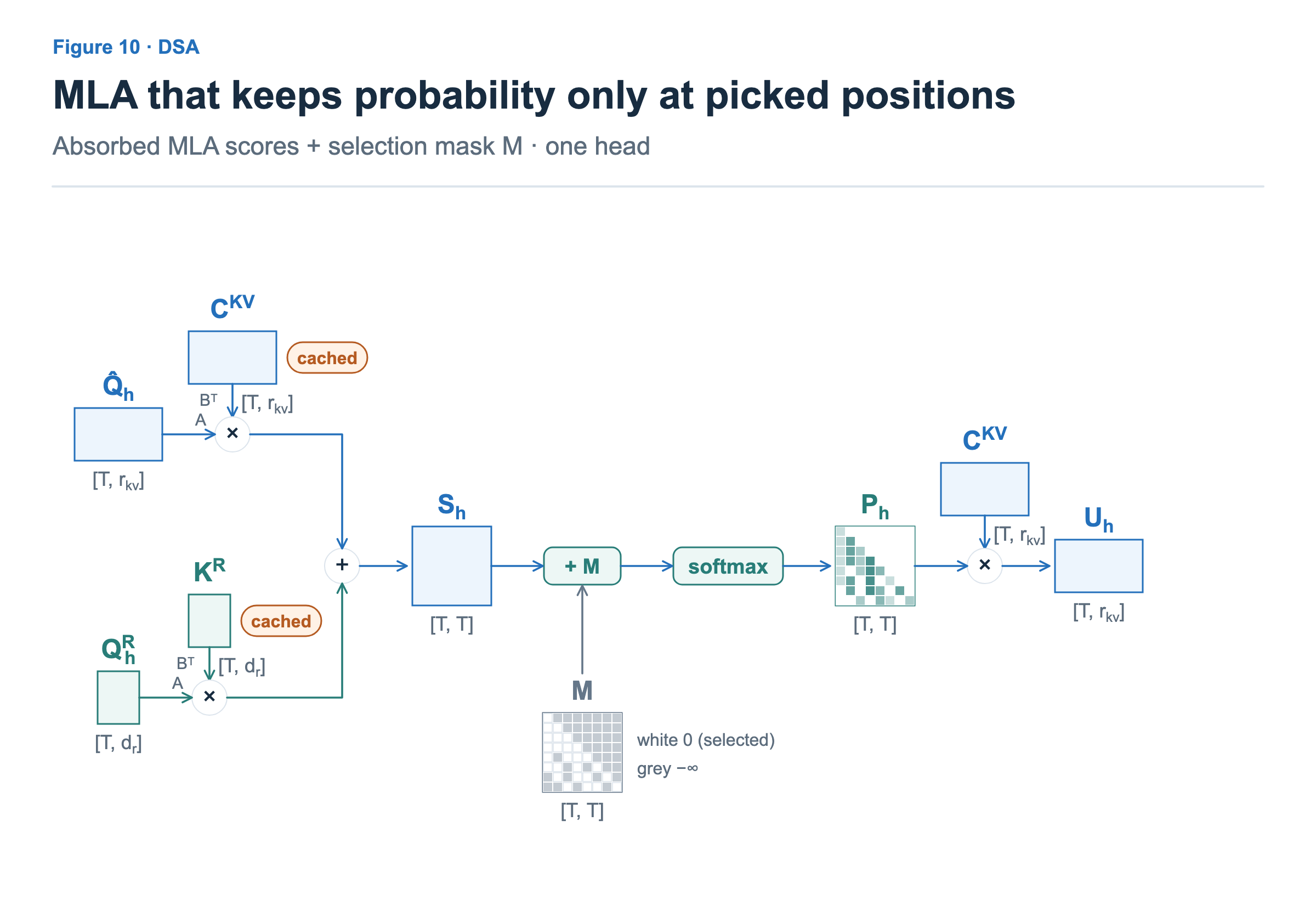
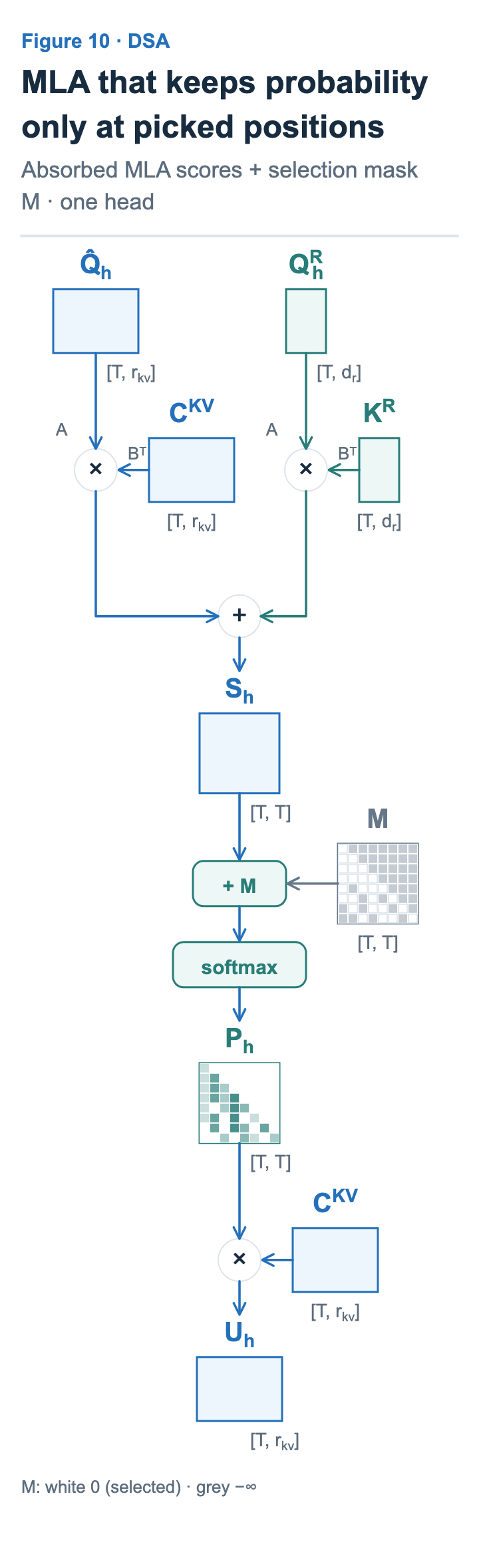
The score is computed exactly as in absorbed MLA. The figure leaves out scaling. M is 0 only at picked positions among those the query can see, so it also does the job of the causal mask.

Adding M to the score makes the probability of unpicked positions zero after softmax.

The figure only expresses the result with a mask. Whether a real kernel reads only the picked positions depends on the implementation. The reads in this article assume an implementation that reads only the KV of the 2,048 picked positions.

Calculating V3.2’s KV cache

Start with the structure alone. What is stored is MLA’s 576 dimensions plus a 128-dimensional search key, 704 dimensions in all. If everything were stored in BF16, that would be 61 layers × 704 × 2 B = 85,888 B, 22% more than V3 (70,272 B). DSA is not a technique for reducing storage. Unpicked positions are not removed from the cache either, because the next token may pick different positions.

Real deployments store at lower precision. For one token in one layer, two groups of values are stored.

Main KV, 656 B. The 512 dimensions of C^KV are stored in FP8 at 1 B per element, 512 B. FP8 has a narrow representable range, so a scale factor for each group of values is stored with it. There is one FP32 scale per 128 dimensions, so 4 × 4 B = 16 B. The 64 dimensions of the positional Key K^R are not quantized and stay in BF16, 64 × 2 B = 128 B. Together, 512 + 16 + 128 = 656 B.

Search key, 132 B. The 128 dimensions of the search key k^I are stored in FP8 for 128 B, with one FP32 scale for all 128 dimensions, 4 B. 128 + 4 = 132 B. The search key is quantized to FP8 entirely, including the dimensions RoPE is applied to; unlike the main KV, no part of it is left in BF16.

Main KV:     C^KV 512 × 1 B + scale 4 × 4 B + K^R 64 × 2 B = 512 + 16 + 128 = 656 B
Search key:  k^I 128 × 1 B + scale 1 × 4 B               = 128 + 4        = 132 B
V3.2: 61 layers × (656 + 132) B = 48,068 B  (about 1/82 of MHA)

Looking at reads

What DSA cuts is what one decode step reads. The right chart of Figure 7 shows what all layers read to generate one token (one decode step) in a 128K context. Each bar is colored in proportion to the KV read by attention (blue) and the search keys read to pick positions (red). Each cache item a layer references is counted once. A cache shared by several layers is counted again for each layer that reads it, but it is not counted twice because of multiple heads in the same layer or the two roles of Key and Value. SWA, scales and padding inside a cache item are included; reading the same values more than once and writes of the new cache are excluded.

This value assumes that only the selected KV and the candidate search keys are read, and computes each cache item’s size in the same deployed cache format as storage. It is a computed amount, not actual memory traffic. The reads if everything were stored in BF16 are collected in the box at the end of this section.

In V3.2, the KV read by attention is 61 layers × 2,048 positions × 656 B ≈ 82 MB. Position selection cuts the positions each layer reads from 131,072 to 2,048, to 1/64, and storing the main KV at lower precision adds to that. In exchange, the indexer scans the keys of every position: 61 layers × 131,072 × 132 B ≈ 1.06 GB. The total is about 1.14 GB, and search keys make up about 93% of it. That alone does not mean picking positions takes most of the execution time, because computation and actual memory access patterns differ.

The indexer is still cheaper than reading every position with the main attention because each key is small (128 dimensions, FP8), every head reads the same key, and there is no softmax, only ReLU and a weighted sum. But it still scans the whole context. Cutting this cost together with storage is the task V4 takes on. How the indexer works is covered in the sparse indexer article.

V3.2:       KV 61 × 2,048 × 1,152 B          search keys 61 × N × 256 B
V4-Flash:   KV (21 × 512 + 20 × N/128 + 43 × 128) × 1,024 B    search keys 21 × N/4 × 256 B
V4.1-Flash: KV (38 × 512 + 40 × 128) × 1,024 B    search keys (3 × N/2 + N + 4 × 16,384) × 256 B
N = 131,072

DeepSeek-V4-Flash

V4 uses compression along tokens: it merges the KV of several tokens and stores the result as one vector. This one compressed vector is called an entry. It mixes two schemes with different compression ratios across layers. CSA (Compressed Sparse Attention) compresses overlapping spans into one entry every 4 tokens and reads selectively with an indexer. HCA (Heavily Compressed Attention) compresses 128 non-overlapping tokens into one entry and reads every completed entry. Recent positions are kept separately without compression. Below we start with HCA, which is simpler, move on to CSA, and then work out the numbers. Figure 11 shows the effect.

Figure 11 · KV cache stored and read: V4-FlashMHA to V4-Flash · several tokens compressed into one entryThe two graphs of the first figure up to V4-Flash, with the V4-Flash row highlighted.

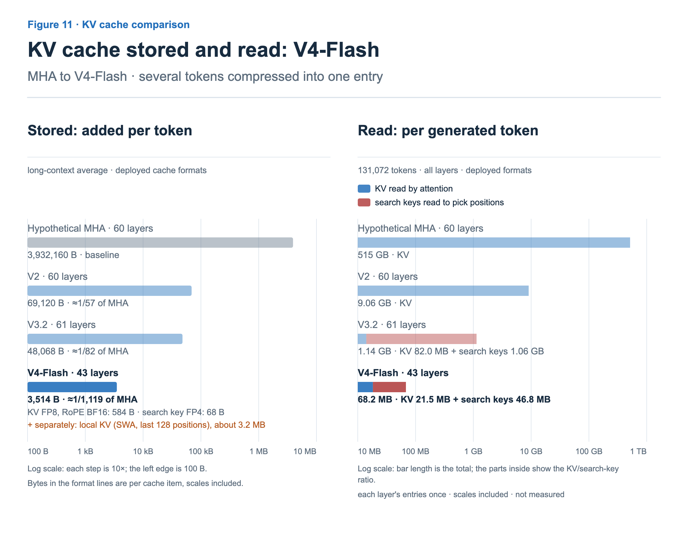
V4-Flash uses about 3,514 B per token. The local KV that keeps recent positions is listed separately in orange.

Reads under the same conditions are about 68 MB.

This article uses V4-Flash as its reference. Of its 43 layers, the first 2 are SWA layers that see only recent positions; 21 are CSA and 20 are HCA. It is also worth noting up front that V4 is not MLA with a compressor added. V4 does not expand per-head Key and Value from a latent the way MLA does. A single 512-dimensional entry serves as both Key and Value for every head. There are no weights like MLA’s W^UK and W^UV that expand Key and Value; each head’s Query is multiplied with the entry directly (Figure 15).

HCA: 128 tokens into one

In this article, the uncompressed KV of the last 128 positions is called the local KV (SWA). SWA (sliding window attention) is attention that reads only the recent positions. What is compressed and built up across a long context splits in two. The compressed KV that attention actually reads is the main KV, and CSA, shown later, adds search keys that pick positions to read. The main KV and search keys together are the global KV. Here “local” refers to the range of recent positions. The V4 report describes the branch that reads recent positions as sliding window attention; the names local KV, main KV, and global KV come from the V4.1 report.

From V4 on, the notation changes a little. c^Q is a small Query latent, like MLA’s C^Q. W^KV_win builds the local KV of the recent window (win), and W^KV_comp builds the candidates to compress (compression). Here C is not MLA’s content part but the candidate values to compress, and Z is not MLA’s head output but the pre-softmax score of each candidate. A finished compressed entry is written C^Comp (compressed).

RMSNorm is a normalization that keeps a vector’s size constant. In Figure 12, c is the width of one entry (512), and an entry of this width serves as both Key and Value. n_h is the number of heads. E^win is a local KV entry of the recent window. Figure 12 leaves out the RoPE step; its form after RoPE is in the comparison part of Figure 13.

An HCA layer builds three branches from the input X.

Figure 12 · Three branches an HCA layer builds from its inputQuery, local KV, compression candidates C and scores Z · purple = learned weightsHCA attention starts from three branches that multiply the input X by weights. The query takes two steps, W^{DQ} then W^{UQ}; recent-token KV uses W^{KV}_{win}; the compression candidate C and its pre-softmax scores Z use W^{KV}_{comp} and W^Z. Box widths follow the order of column sizes.

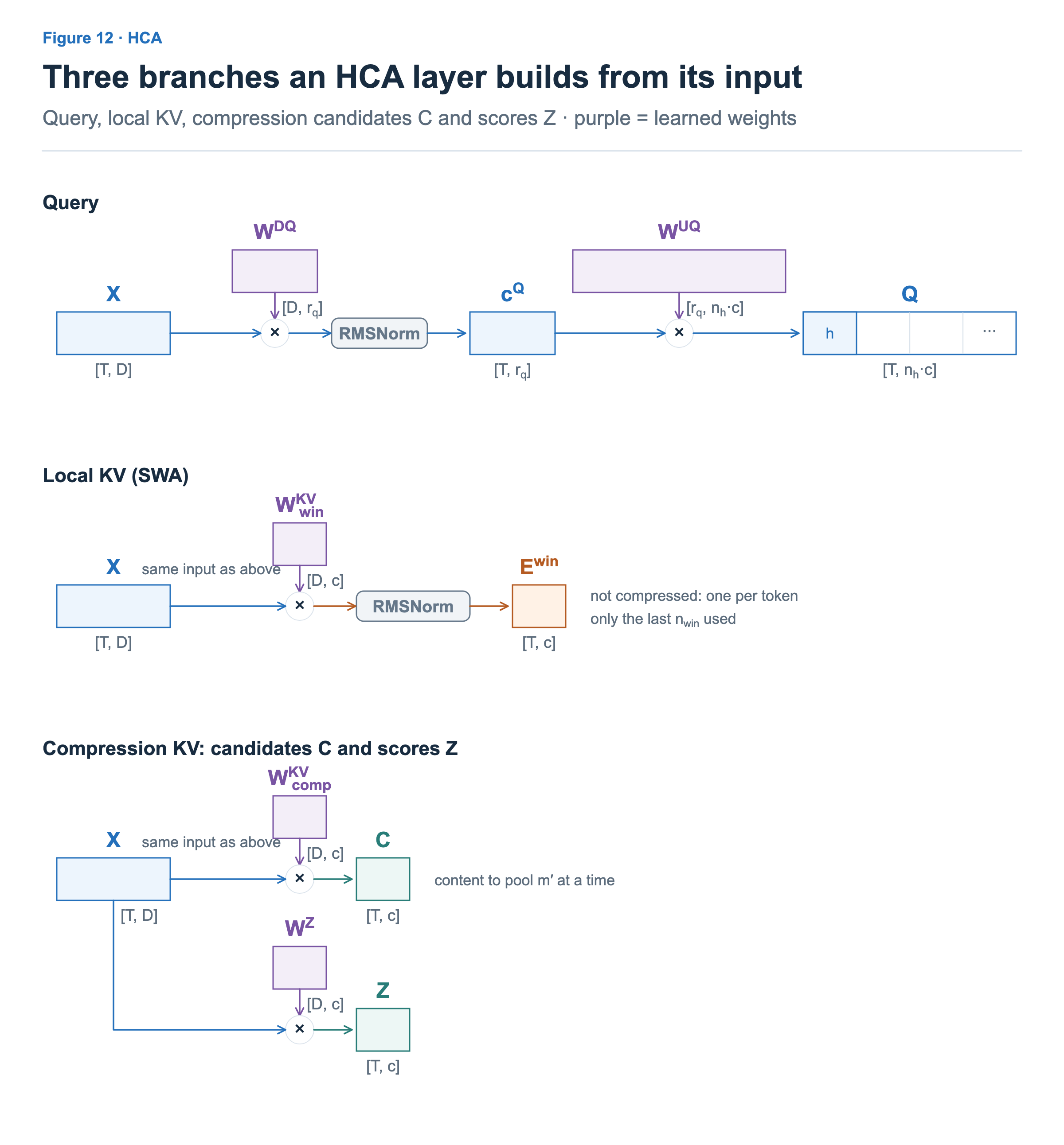
Query. Built through a latent c^Q, as in MLA.

Local KV. Built one per token without compression, keeping only the last 128.

Compressed KV. Builds candidates C and scores Z, then merges m′ tokens into one entry.

Compression is a weighted average computed separately for each channel (one feature column). In the figure, the subscript b is the block number (a block is the m′ tokens compressed together), S_b the weights set by softmax, and u_b the merged row. For teaching, m′ is reduced to 4; a real HCA layer uses m′ = 128.

Figure 13 · Building a compressed entryPer-channel weighted sum over a block · m′ = 4 exampleA compressed entry is a per-channel weighted sum of the block’s four candidate rows C. Scores Z plus position bias B are softmaxed across tokens into S, which weights C; the sum over tokens is passed through RMSNorm and RoPE to give the entry. Recent-token KV is built with a separate weight and no compression.

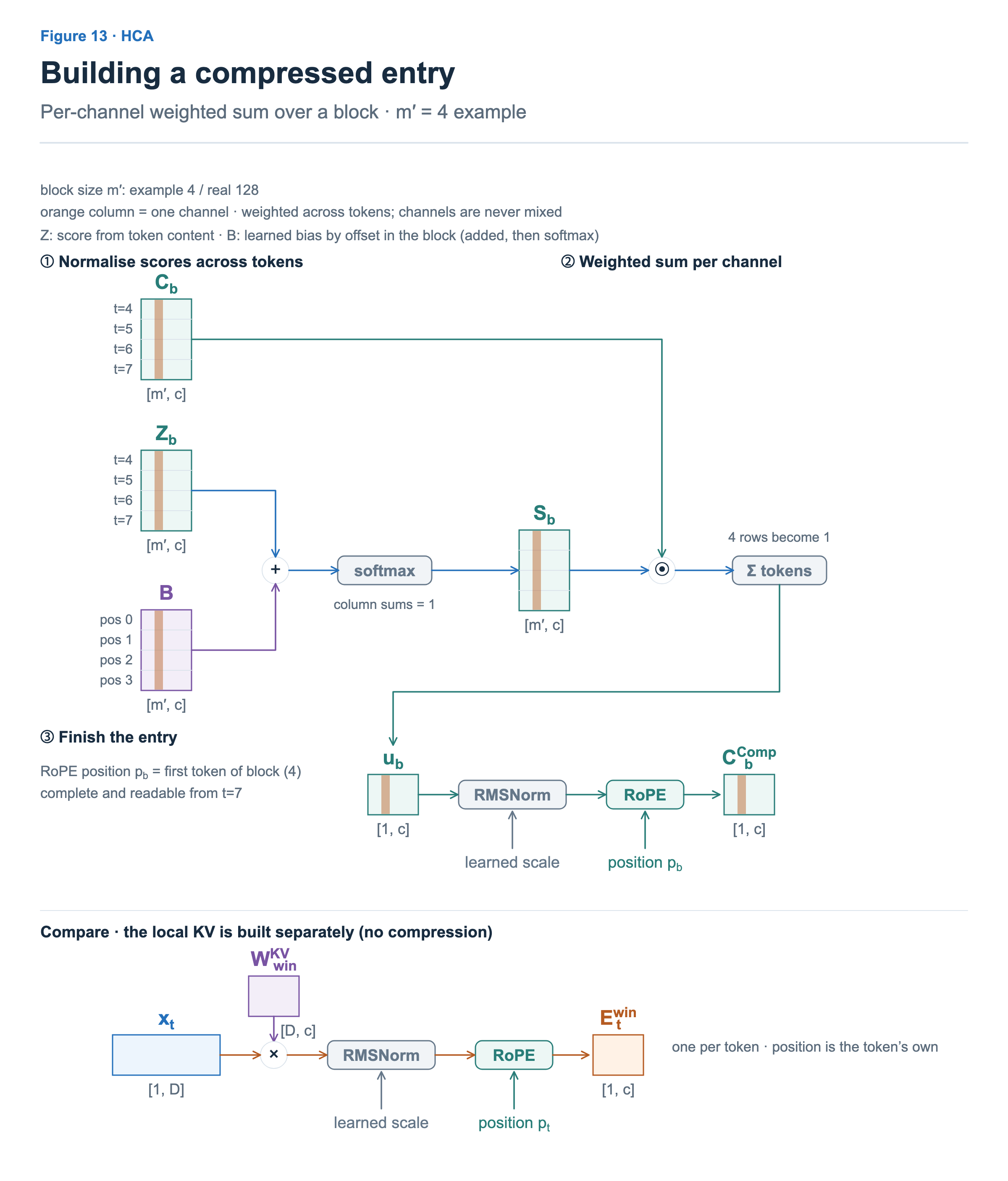
①② Set the weights and merge. The position bias B is added to the scores Z of the tokens in the block, and a softmax along the token direction sets the weights. B is a value learned for each position (offset) within a block, and every block uses the same B. Merging the candidates C channel by channel with those weights leaves one row.

③ Finish the entry. The merged row goes through RMSNorm and RoPE to become an entry. An entry is complete only once its block is full. The ‘learned scale’ in the figure is a learned weight multiplied after RMSNorm, not the scale used for FP8 storage. RoPE is applied only to the last 64 dimensions of an entry.

Compare. The local KV is built separately for each token, without compression.

A compressed entry can be read only once its block is full. Figure 14 shows how the entries a token can read change as one more token arrives.

Figure 14 · Entries readable right nowCompleted compressed blocks plus the recent window · t=6 vs t=7Token t reads the completed compressed blocks plus the recent window including itself. At t=6 only block 0 is complete (5 rows); at t=7 block 1 completes (6 rows), and a compressed entry and a window entry may cover the same source tokens.

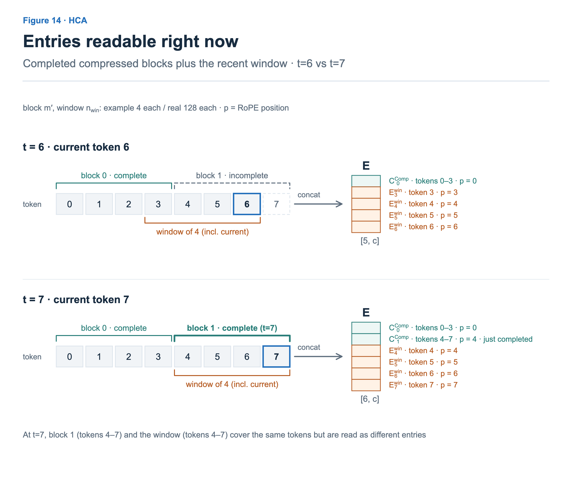
t = 6. Token t reads all completed compressed entries concatenated with the recent window, which includes the current token. Here only block 0 is complete, and the recent tokens of the still incomplete block 1 are read through the window.

t = 7. Block 1 is now complete too, adding one compressed entry. The window is read as well, so the same original token can appear in both a compressed entry and a window entry.

Attention then uses the entries gathered this way as both Keys and Values.

Figure 15 · Attention over a shared K = VThe readable entries E serve as Key and Value, then a grouped output projectionAfter per-head normalisation and RoPE of the query, the visible entries E serve as both K and V. S = Q·Eᵀ/√c goes through a softmax with the sink added to the denominator to give P, P·E gives the head outputs O, which get an inverse RoPE. Heads are grouped, each group uses its own W^{O,a}, and a shared W^{O,b} maps back to the hidden size.

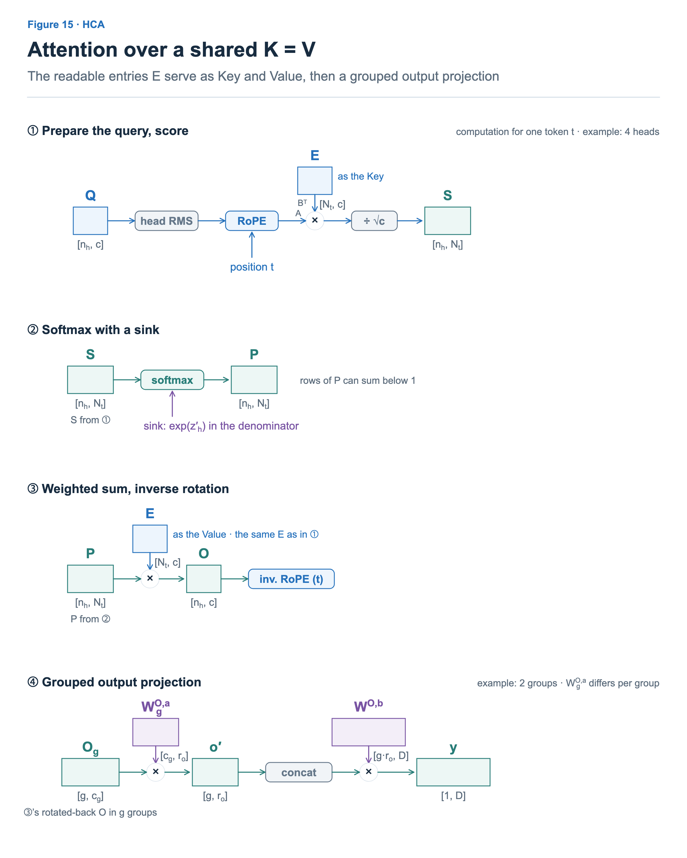
① Prepare the query, score. The query is normalized per head with RMSNorm (head RMS) and rotated with RoPE for position t, then multiplied with the N_t entries E gathered in Figure 14 to give the scores S. Here E plays the Key role. There are no weights that expand per-head Key and Value.

② Softmax with a sink. Each head adds exp(z′ₕ), from a learned value z′ₕ, to the softmax denominator, so the weights on the real entries can sum to less than 1. This value, the sink, leaves room to pay less attention to every entry.

③ Weighted sum, inverse rotation. The probabilities P weight the same E, now as the Value, giving the head outputs O. E serves as the Value with RoPE still applied, so the last 64 dimensions of the output are rotated back by the current query position t (inverse rotation). The entry at position s had been rotated by s, so after the inverse rotation each entry’s contribution is rotated by s − t: by relative distance rather than absolute position. The reasoning is in the ‘RoPE’s rotation’ box in the V2 section.

④ Grouped output projection. The heads of O, rotated back in ③, are put into g groups. The width of one group, c_g, is the outputs of its heads concatenated. Each group is reduced to width r_o with its own W^O,a_g, the results are concatenated, and a shared W^O,b maps them back to the hidden size D.

Since Key and Value are the same entry, it only needs to be stored once.

CSA: compress with overlap and read selectively

CSA adds two things to the same frame as HCA. Compression spans overlap, and an indexer picks which entries to read.

Figure 16 · Where a CSA layer differs from HCAOverlapping compression (candidates twice as wide) and the indexerA CSA layer has query, local-KV and output weights with HCA’s structure, plus twice-as-wide overlapping-compression weights (the a|b halves of W^{KV}_{comp} and W^Z) and an indexer. The indexer takes X and the c^Q shared with the main query and returns the block ids to select.

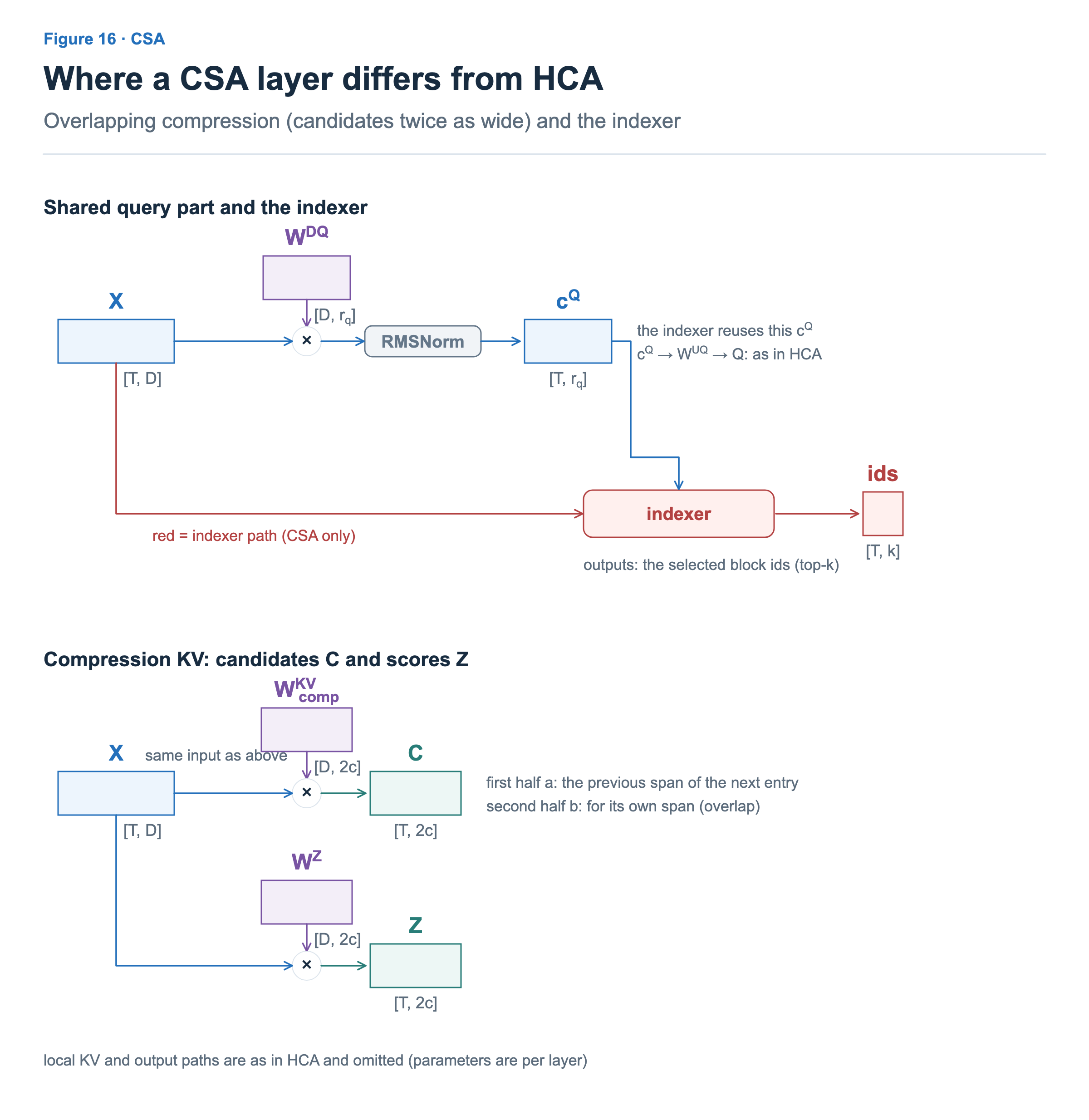
Query and indexer. The Query path is the same as in HCA. The new indexer projects the Query latent it shares with the main attention to build the indexer query.

Compressed KV. The weights for candidates C and scores Z are twice as wide as in HCA, because each span is compressed with an overlap into its neighbor.

Why the candidate weights are twice as wide shows up in how one entry is built. W^KV_comp and W^Z give each token candidates and scores 2c wide, used as a first half a and a second half b. The second half b goes into the entry of the token’s own span, and the first half a goes into the entry of the next span as its ‘previous span’. So one entry gathers 8 rows, a from the 4 tokens of the previous span and b from the 4 tokens of its own span, and merges them the same way as HCA. The softmax over these 8 rows’ scores, with the position bias added, gives the weights used for compression.

Figure 17 · Building an entry with overlapping compressionPrevious span a + own span b, one softmax over 8 · m = 4A CSA entry reads eight tokens: four of the previous span (a) and four of its own span (b). Scores Z plus the per-span, per-offset bias B are softmaxed once across the eight tokens, weight the candidates C, are summed, then get RMSNorm and RoPE (position = the start of its own stride span). Neighbouring entries share half their span.

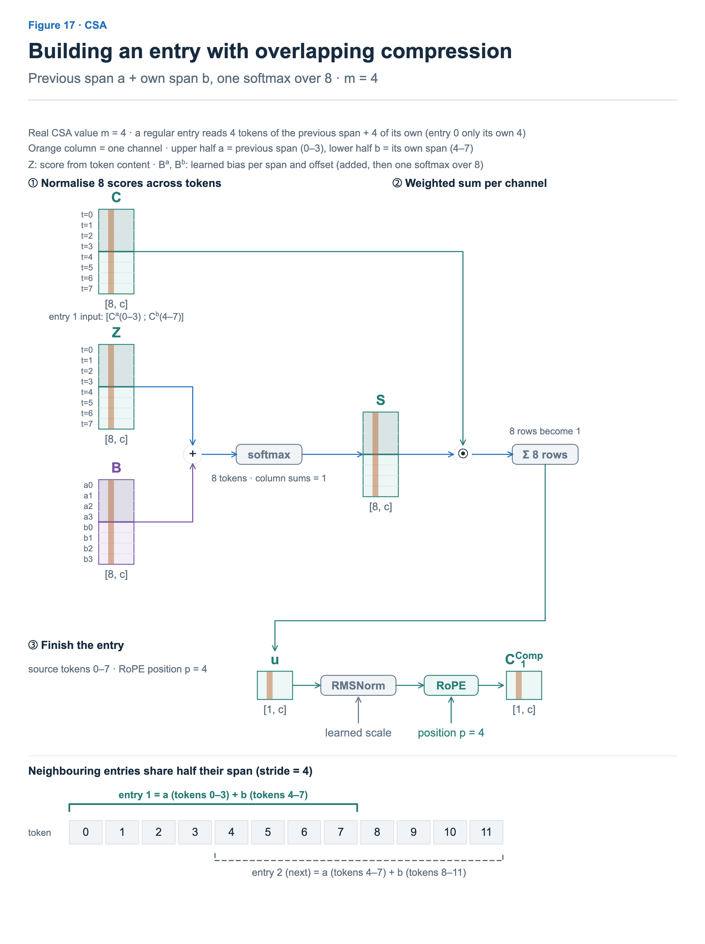
①② One entry from 8 tokens. One CSA entry reads 8 tokens: the 4 tokens of its own span (b) and the 4 of the previous span (a). m = 4 is CSA’s real value.

③ Finish the entry. Even so, one entry is produced every 4 tokens. The compression ratio is 4, so the number of stored entries is 1/4 of the number of tokens. As in HCA, an entry’s RoPE position is the first token of its own span (p = 4 in the figure); reading the previous span as well does not change that.

Neighboring entries. Neighboring entries share half of their source tokens, so information from both sides of a block boundary can be reflected. This is weighted compression, so it does not mean the information is preserved as is, and the first entry has no previous span.

CSA reads only some of the compressed entries, so it needs an indexer to decide which ones.

Figure 18 · Indexer: scoring and picking blocksOwn compressed keys · shared query latent · head weights → ReLU-weighted sum → top-kThe indexer builds candidate keys K^{IComp} with a compressor separate from the main one, scores each completed block with I[t, s] = Σ_h w_h · ReLU(q_h · K_s) using q^I (raised from the same c^Q as the main query) and the head weights w^I, and picks the k best block ids. Those ids point at the main compressed entries.

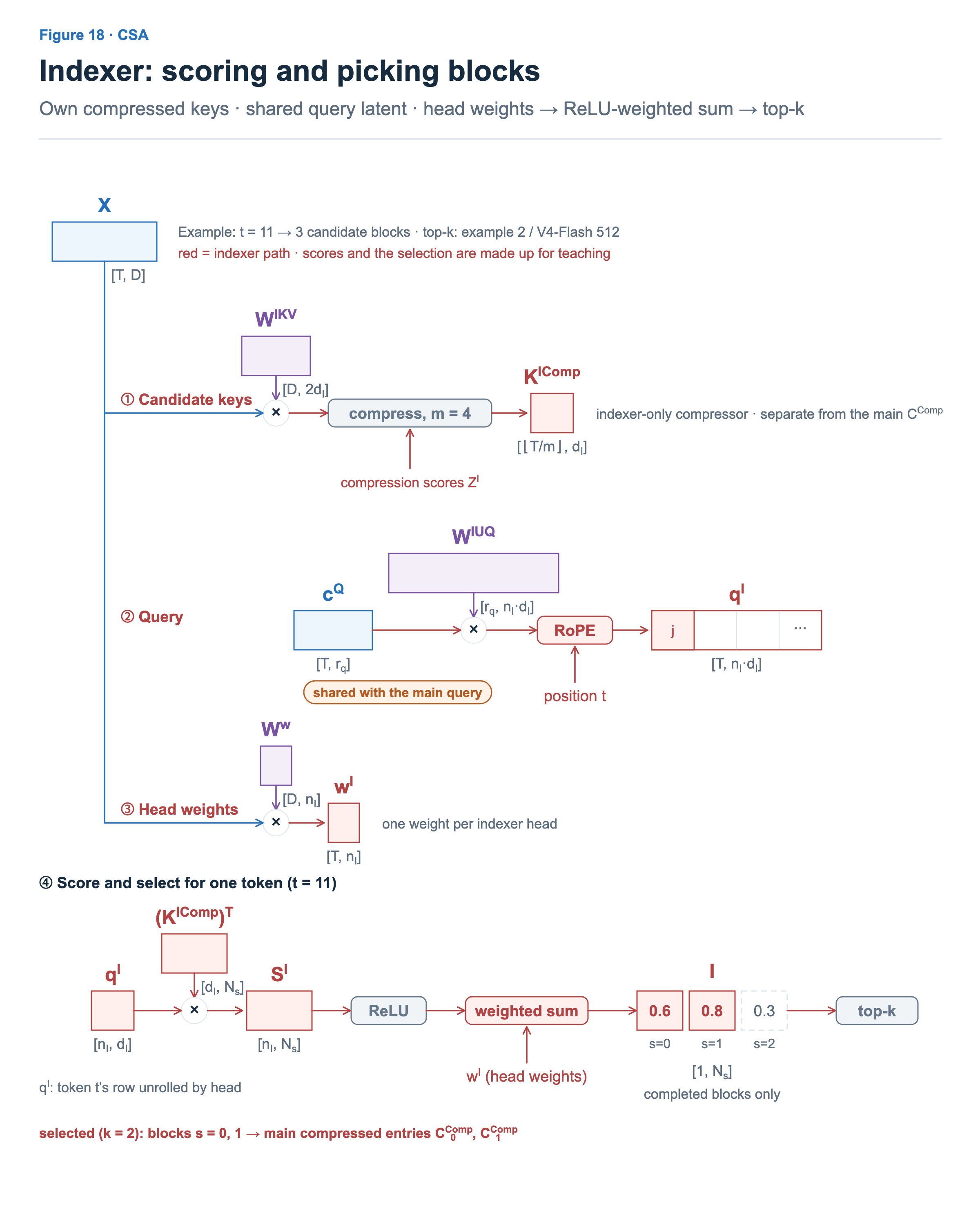
①②③ Key, query, head weights. In the figure, n_I is the number of indexer heads, d_I the width per head (the same as V3.2’s H^I and d^I), and N_s the number of compressed entries completed so far. CSA’s indexer uses the same score formula as V3.2’s, but builds its keys with a separate compressor. So search keys are also stored one per 4 tokens, with 128 dimensions. This compressor builds its own candidates and scores Z^I from X the same way as the main compressor and builds one entry per 4 tokens with the same overlap, so search key s and main entry s stand for the same span of original tokens.

④ Score and select. Scores are combined with the head weights, and the highest-scoring blocks are picked for each token. Blocks not yet complete at that query position are not candidates.

Adding the recent window to the picked compressed entries settles what this token reads.

Figure 19 · Entries actually readCompressed entries picked by the indexer + the recent window · t = 11Token t reads the k highest-scoring completed compressed entries plus the recent window including itself. At t = 11 three candidates are complete and only the best two are read, so the newly completed entry is not necessarily chosen.

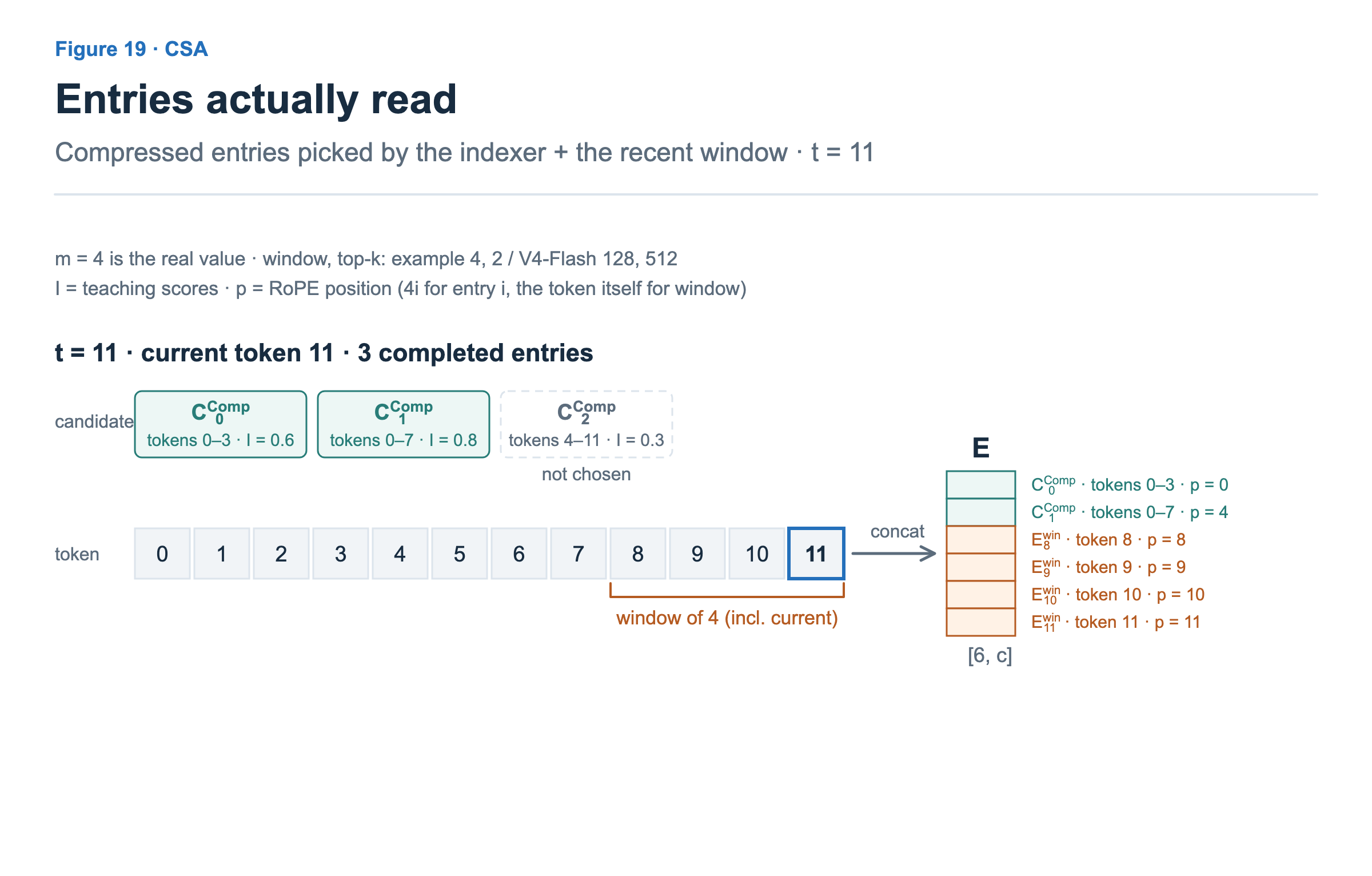
Token t reads the k compressed entries picked by the indexer plus the recent window. This differs from HCA, which reads all compressed entries.

HCA compresses 128×, so there are few entries and reading them all is fine. CSA compresses 4×, so there are many entries, and it reads selectively.

Calculating V4-Flash’s KV cache

CSA layers store a 512-dimensional main KV entry and a 128-dimensional search key every 4 tokens, and HCA layers store a 512-dimensional main KV entry every 128 tokens.

On structure alone, even if everything were stored in BF16, that is 21 × 640 × 2 B ÷ 4 + 20 × 512 × 2 B ÷ 128 = 6,880 B, about one-tenth of V2. The width of the stored vector (512) is close to MLA’s 576, but 4 and 128 tokens are compressed into one entry.

The deployed format stores main KV entries mostly in FP8 and search keys in FP4. The format used in this article is 584 B per main KV entry and 68 B per search key.

V4-Flash: 21 layers × (584 + 68) B ÷ 4 + 20 layers × 584 B ÷ 128 ≈ 3,514 B  (about 1/1,119 of MHA)

Main KV entry: 448 non-RoPE dims × 1 B (FP8 E4M3) + 64 RoPE dims × 2 B (BF16)
               + one UE8M0 scale per 64 channels, 1 B × 7 + padding 1 B = 584 B
Search key:    128 dims × 0.5 B (FP4 E2M1)
               + one UE8M0 scale per 32 channels, 1 B × 4 = 68 B

On top of this there is a separate local KV cache. All 43 layers keep the KV of the last 128 positions without compression. In the deployed format that is 43 × 128 × 584 B ≈ 3.2 MB. This value stops growing once the last 128 positions are filled. But as the per-token growth shrank, local KV became a larger share of storage. Approximating global KV as per-token growth × context length, the two are about equal at roughly 900 tokens. For shorter contexts, the local KV cache is larger. The approximation ignores rounding of compressed blocks and intermediate compression state.

Reads (the right chart of Figure 11) also dropped. The KV read by attention is about 21.5 MB, and the keys read by the indexer about 46.8 MB. The KV is (21 CSA layers × (512 picked + 128 window) + 20 HCA layers × (N/128 + 128) + 2 SWA layers × 128) cache items at 584 B each, since compressed entries and uncompressed window positions are stored in the same format. That is far less than V3.2’s 1.06 GB because search keys are compressed 4×, only 21 layers use the indexer, and each key shrinks from 132 B to 68 B. HCA layers read every compressed entry, so that part keeps growing in proportion to context.

DeepSeek-V4.1-Flash

V4.1 changes compression and selection with CSA2 and shares KV and selection lists across layers. This brings the number of layers that store global KV down to four, and storing main KV in FP4 also cuts storage. In addition, the CED (Causal Encoder–Decoder) structure, together with an approximation that recomputes only the recent span, reduces prompt-processing compute. The 40 layers of V4.1-Flash split into the first 20 (encoder) and the last 20 (decoder). This is a different structure from the encoder–decoder of a translation model; the CED section looks at it in detail. Figure 20 shows the effect.

Figure 20 · KV cache stored and read: V4.1-FlashMHA to V4.1-Flash · sharing cuts the layers that storeThe two graphs of the first figure up to V4.1-Flash, with the V4.1-Flash row highlighted.

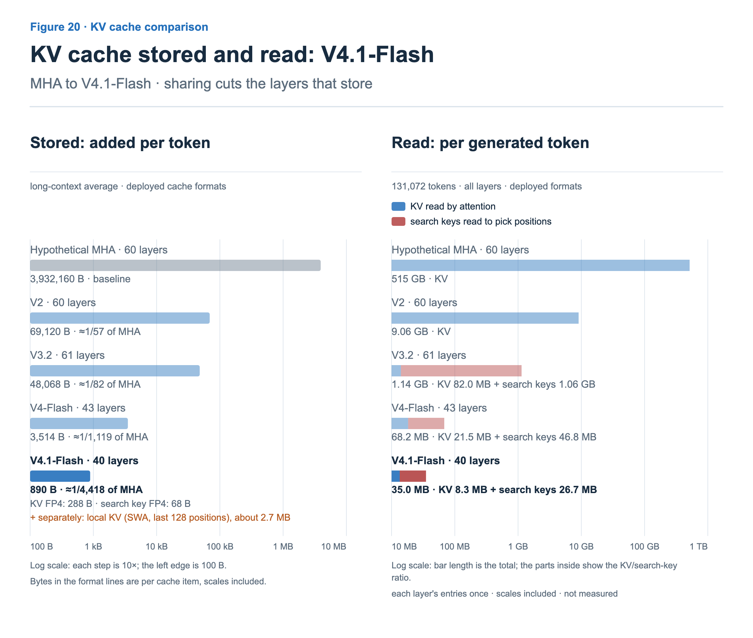
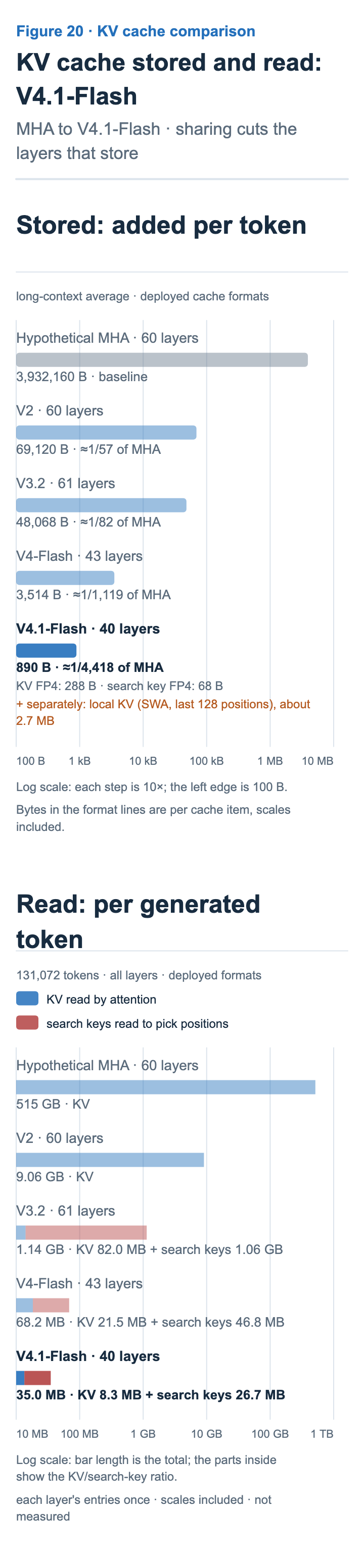
V4.1-Flash uses 890 B per token, about 1/4,400 of the hypothetical MHA.

Reads under the same conditions are about 35 MB.

CSA2: compression without overlap, and the search key

CSA2 changes two things within a layer. Compression spans no longer overlap, and the search key is built from the main KV instead of by a separate compressor.

Figure 21 · CSA2 compresses without overlapComparison m = 4 (real CSA2: encoder m = 2, decoder m = 1) · tokens behind entry 1 and the softmax sizeCSA builds an entry from 8 tokens, the previous span a and its own span b, so neighbouring entries share half their span; the compressor has an absolute in-span position bias B and one softmax over 8. CSA2 removes the overlap and B: an entry comes from the m tokens of its own span only, with one softmax over m.

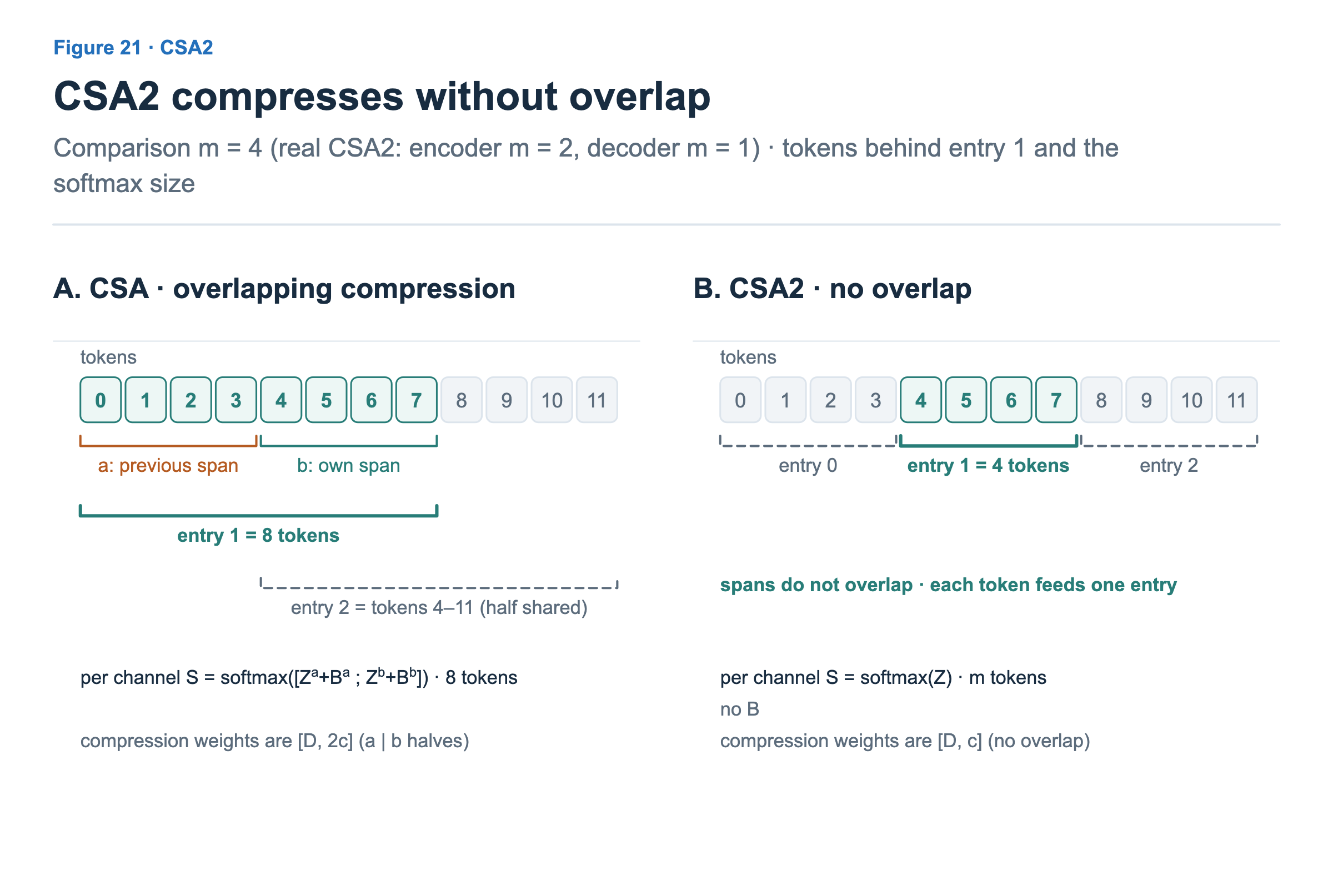
CSA. One entry reads its own span together with the previous span, sharing half of its tokens with the neighboring entry.

CSA2. Spans do not overlap, so each token goes into exactly one entry. The position bias B inside the compressor is gone as well.

The compression ratio also dropped. In real CSA2, encoder layers pack 2 tokens into one entry (m = 2), and decoder layers build one entry per token without compression (m = 1). The ‘pooling’ in Figure 22 is the same compression as the channel-wise weighted average in Figure 13. With m = 1 there is only one token to pool, so the pooling step of Figure 22 passes it through unchanged.

Figure 22 · CSA2 builds the indexer key from the main KVCSA: two compressors from X · CSA2: one compressor and one projectionCSA runs two separate overlapping compressors on the same input X to make the main KV and the indexer key. CSA2 builds the main KV with a single compressor that has no overlap and no absolute positional embedding B, and builds the indexer key by projecting that main KV (after RMSNorm, before RoPE) with W^{IK} and normalizing it.

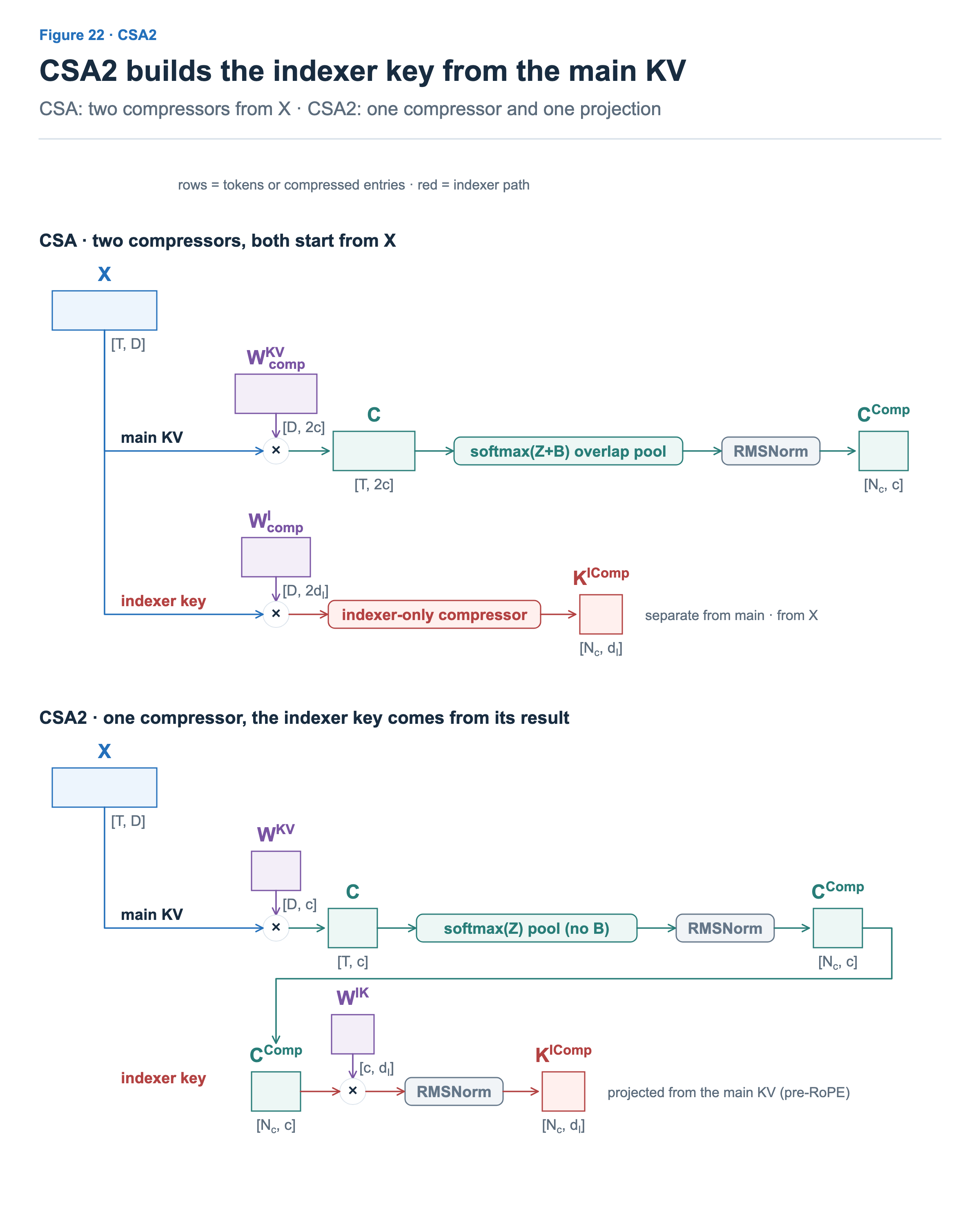
CSA. The compressor ran twice on the same input to build the main KV and the search key separately.

CSA2. There is only one compressor. Its output after compression and RMSNorm, before RoPE, is projected and normalized to build the search key. RoPE is then applied separately to the main KV and the search key. N_c in the figure is the number of finished compressed entries, the same as N_s in Figure 18. So only in Figure 22 is C^Comp the value before RoPE; in the other figures C^Comp is the entry after RoPE.

Because both come from the same entry, they are easier to pass along together in the cross-layer sharing shown next.

Sharing KV across layers: Full, Reindex, Reuse

Until now, every layer stored its own KV. In V4.1-Flash, four Full layers build and store global KV, and the remaining CSA2 layers share it. The first two layers use SWA only, and all 40 layers build their own local KV.

Each CSA2 layer is fixed to one of three modes.

Figure 23 · Three modes of a CSA2 layerWhat a layer builds and what it borrowsA CSA2 layer is Full, Reindex or Reuse. Full builds the compressed KV and the indexer keys and selects the top-k KV rows with its own indexer query. Reindex borrows the KV and indexer keys from the latest Full layer and reselects with its own indexer query. A Reuse layer has no indexer: it borrows the KV and the latest Full or Reindex selection. All three join the k selected rows with their own window KV and compute attention with their own query.

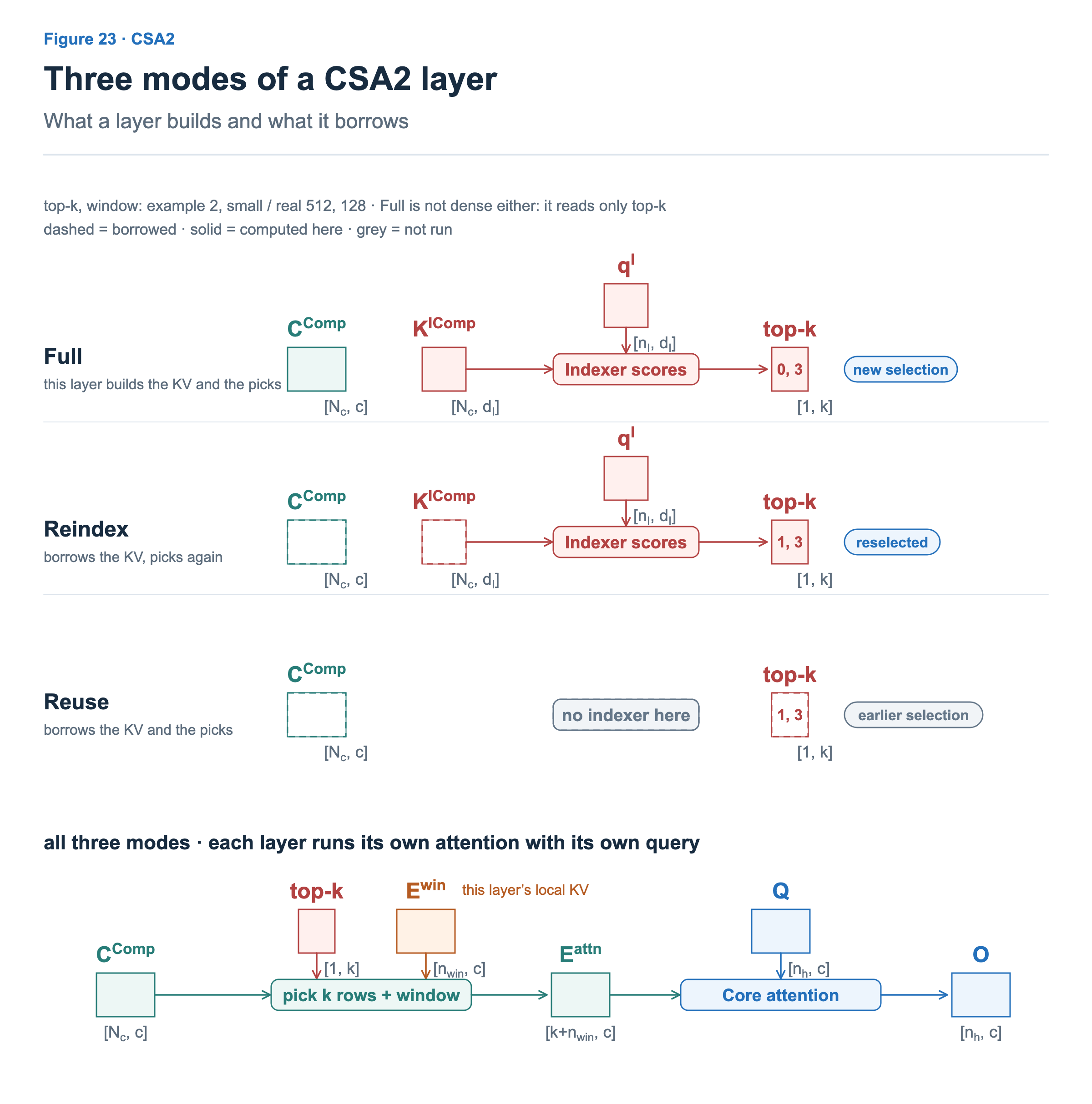
A Full layer builds new main KV and search keys and picks its top-k with its own indexer. Only Full layers store global KV. Full is not dense attention over every position either; it reads only the top-k.

A Reindex layer borrows the main KV and search keys of the most recent preceding Full layer and picks positions again with its own indexer query.

A Reuse layer has no indexer. It borrows both the main KV and the selection list from earlier layers.

Common to all three modes. The picked main KV rows are joined with this layer’s local KV, and attention is computed with this layer’s Query. The figure draws it once, but every layer computes it on its own.

What is shared is the global KV and the selection list, not the result of attention. Sharing works even though each layer’s representation differs because the model is trained from the start with this sharing. The principle of cross-layer sharing is covered in the cross-layer KV sharing article.

The layout of the 20 encoder and 20 decoder layers is shown in Figure 24.

Figure 24 · The 40-layer layout of DeepSeek-V4.1-Flashencoder 2 SWA + 18 CSA2 · decoder 20 CSA2 · KV groups differ from selection groupsIn the encoder the first two layers use SWA only and the other 18 are CSA2 layers (compression 2) in three groups of [Full, Reuse×5]. The 20 decoder layers are CSA2 layers (compression 1): the first group is [Full, Reuse×3] and four more groups are [Reindex, Reuse×3]. The decoder has a single main KV, built by its first Full layer, and five selection lists: one from Full and four from Reindex.

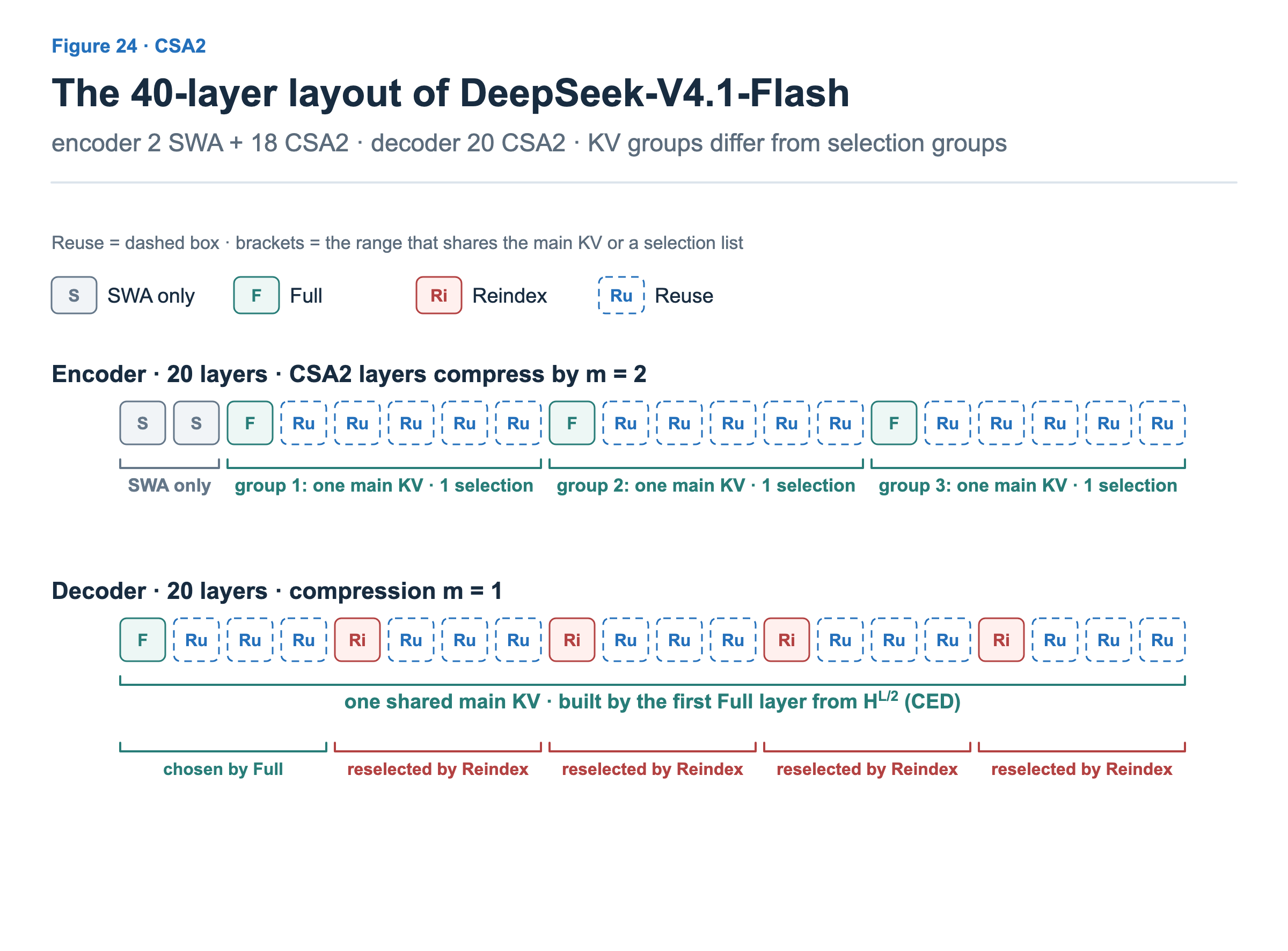
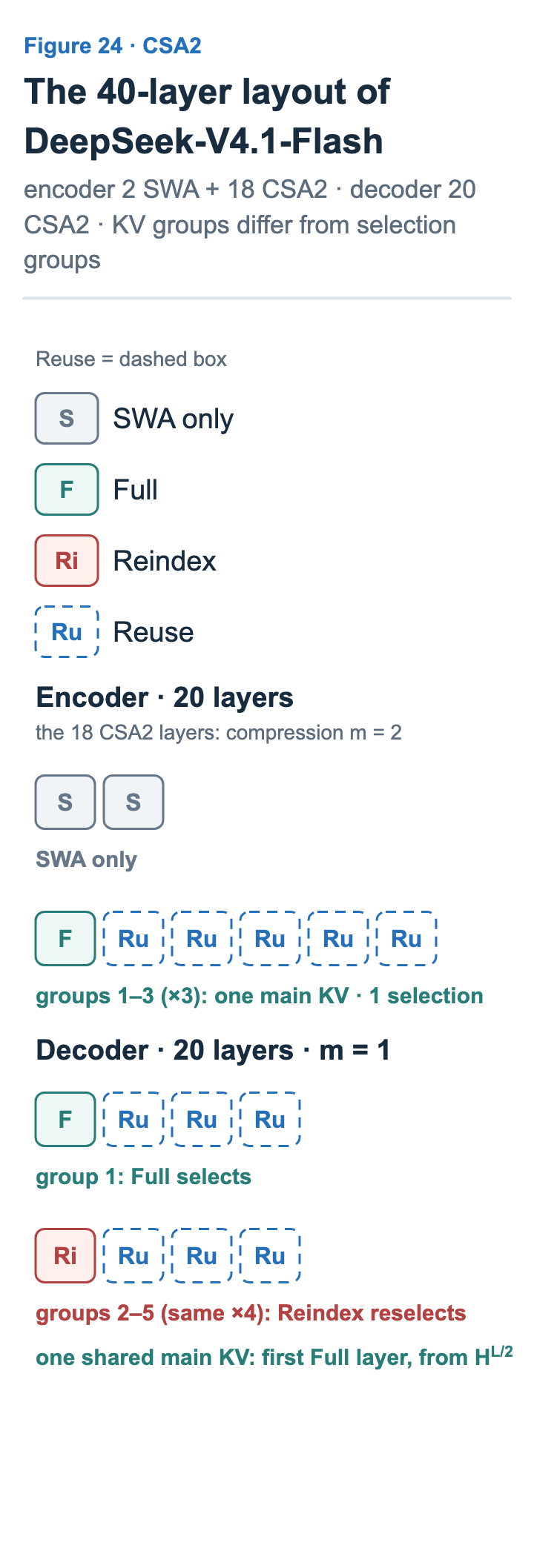
Encoder. The first 2 layers use SWA only, and the remaining 18 form three groups of [Full, Reuse×5].

Decoder. The global KV for all 20 layers is built by only the first Full layer, and four Reindex layers pick positions again. H^L/2 in the figure is the output after the 20 encoder layers.

In the end, 4 layers store global KV: 3 Full layers in the encoder and 1 in the decoder. In the decoder, the cost of picking is also bounded by a hierarchical indexer. Figure 25 shows the hierarchical selection scheme the report introduced in later training. Here a block is a grouping for search, not compression: the decoder’s main KV has one entry per token (m = 1), and 8 consecutive entries form a block whose candidates are picked by the block’s maximum score.

Figure 25 · A hierarchical indexer: narrow the pool, then pick againdecoder only · the first Full layer builds a candidate pool and later Reindex layers score only inside itThe hierarchical sparse indexer is used only in the decoder. For one query the first Full layer scores every causally visible main-KV position, picks its own top-k, and builds a candidate pool from the blocks with the largest block-max scores. Later Reindex layers score only positions in the pool and pick their own top-k; Reuse layers score nothing and reuse the latest selection. The pool is larger than the final top-k.

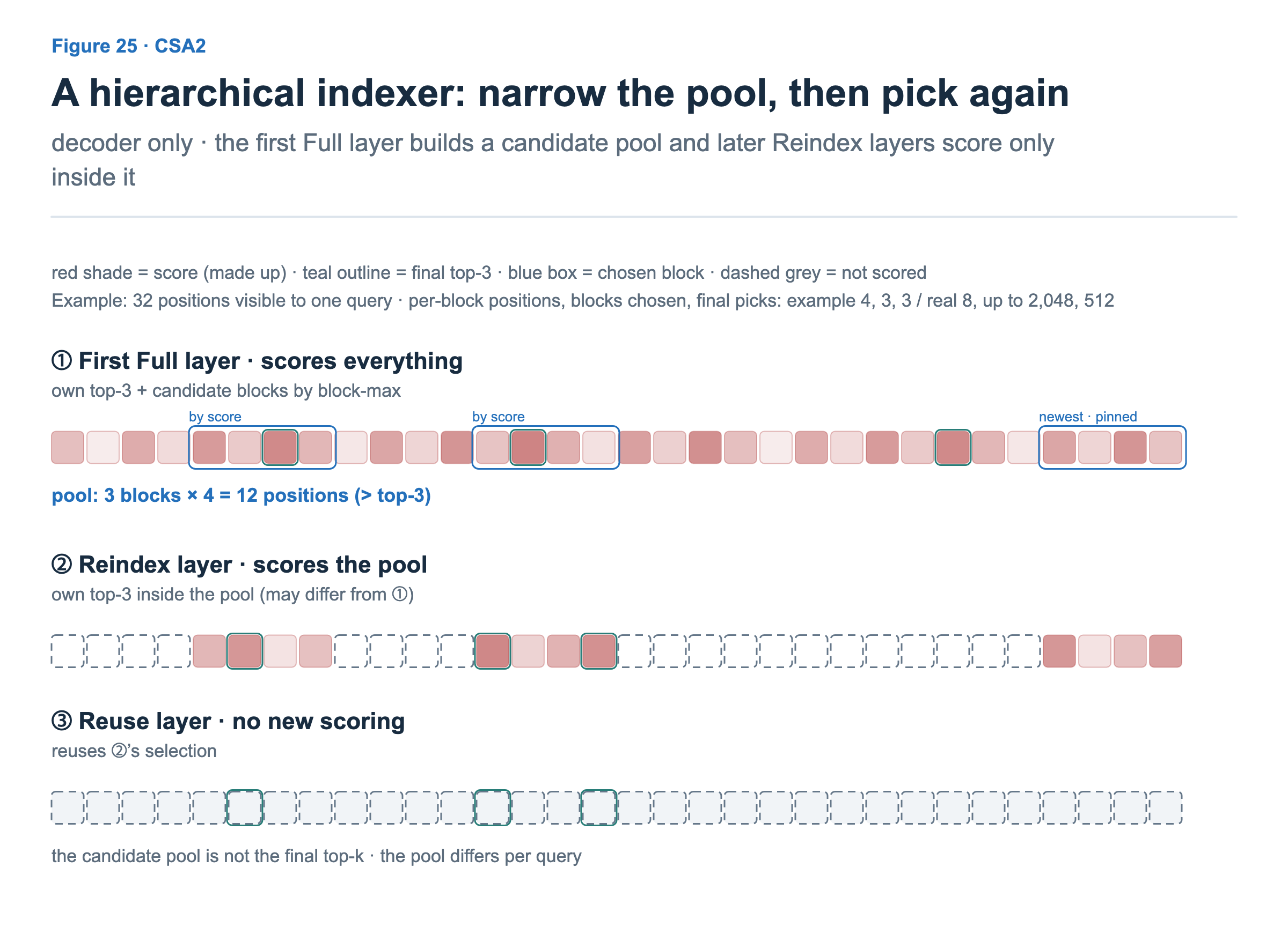
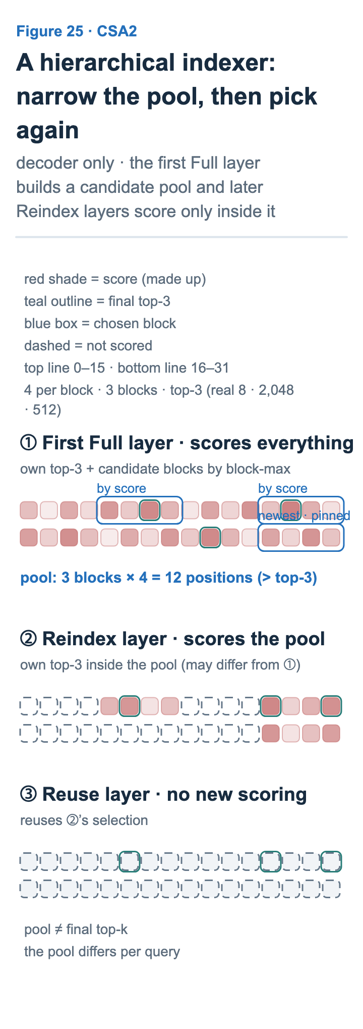
① First Full layer. It scores every position to pick its own top-512, and at the same time picks high-scoring blocks to build a candidate pool (up to 2,048 blocks × 8 positions = 16,384 positions per query). The block holding the query’s newest position, marked ‘newest · pinned’ in the figure, always goes into the pool regardless of its score. This block counts within the 2,048 blocks (one of the three in the figure). The first Full layer picks its top-512 over all positions separately, so its picks can include positions outside the pool it passes to later layers.

② Reindex layer. In this hierarchical scheme, it scores only within this pool and does not scan the whole context again.

③ Reuse layer. The Reuse layer in this example uses the selection of the ② Reindex layer as is. In general, it reuses the selection of the most recent Full or Reindex layer.

The cost of the first Full layer scanning the whole context remains.

CED: the decoder’s global KV comes from the encoder

V4.1’s encoder and decoder both process the same token sequence causally. In decode, the current token passes through the 20 encoder layers and then the 20 decoder layers in turn. This structure is called CED (Causal Encoder-Decoder). The difference lies in where the KV that decoder layers read is built.

Figure 26 · A decoder layer reads KV from two sources with its own queryglobal KV from the encoder output · query and local KV from this layer · CED as run in the reportLeft: encoder layers 1–2 and decoder layers 1–2 stacked upwards. The encoder output feeds the shared global KV (main KV and search keys) on the right. The zoom box shows decoder layer 2: its input splits into its main query and local KV, and the main query reads the main KV entries picked with the search keys together with the local KV, then takes a weighted sum.

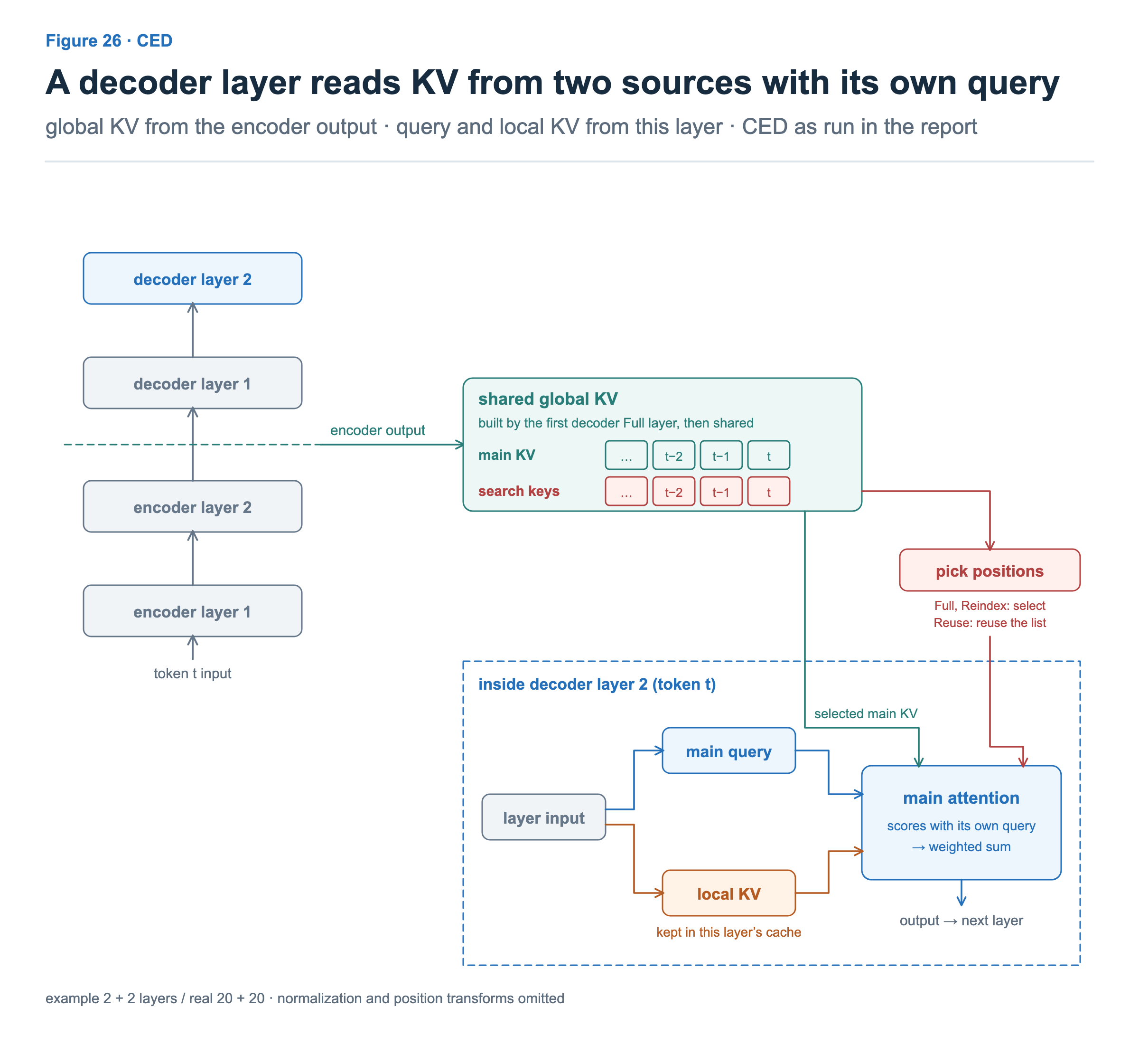
Left: the layer stack. Token t passes through the layers from bottom to top. The decoder’s global KV (main KV and search keys) is built not from the decoder’s own hidden states but from the encoder’s final output. The first decoder Full layer projects this output to build it, and the other decoder layers share it.

Right: inside one decoder layer. This layer builds the main Query and local KV from its own input. It then concatenates the main KV at positions picked with the search keys and its own local KV, scores them with its own main Query, and takes the weighted sum. Separately, the Full and Reindex layers score positions for selection with their own indexer query.

Even when several layers share the global KV, the Query that reads it differs from layer to layer.

This split makes it possible to cut compute in prefill, where the prompt is processed.

Figure 27 · CED prefill: the decoder runs only the recent window, approximatelya prompt without cache reuse · runs upwards · bounded replay per the reportA grid of 8 positions and 4 layers. Encoder layers 1 and 2 run on every position. The encoder output builds the global KV for every position. Decoder layers 1 and 2 run only the last two positions to prepare local KV; the other six are skipped. The running decoder cells read selected global KV entries.

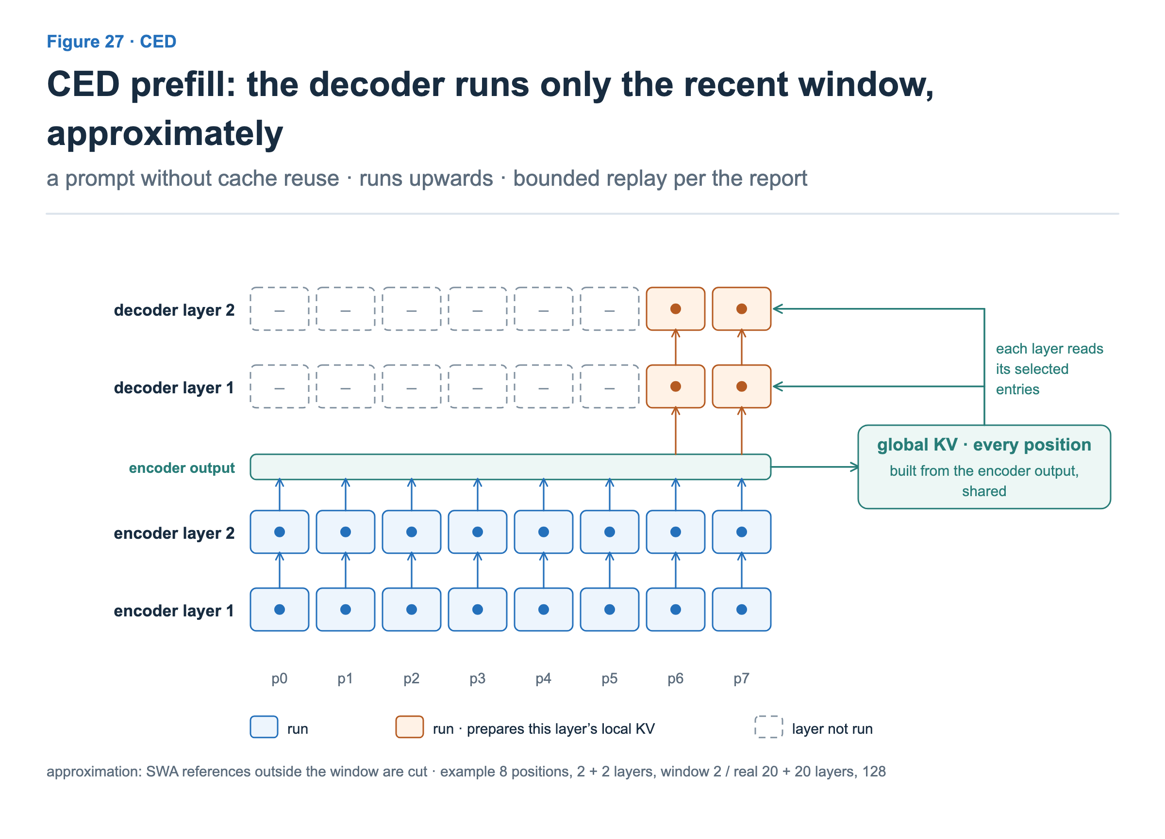
Encoder layers run over every position of the prompt. Their output builds the global KV that the decoder reads, for every position.

The only cache left to prepare by running the decoder is each decoder layer’s local KV, and local KV needs only the last 128 positions. So decoder layers run only over the positions in the recent window. The report calls this run replay. The decoder has not passed over those positions before; the name means only the recent span is sent through the decoder. The decoder output at the last prompt position gives the first token, and after that decode runs all 40 layers.

Replay does more than project KV. It passes the recent positions through the decoder layers in order, running attention and the FFN as well. The first decoder layer takes the encoder output at those positions, each later layer takes the output of the decoder layer just below it, and during the run each layer also reads its selected entries from the global KV.

For long prompts, the number of (position, layer) evaluations in prefill is roughly halved, since the 20 decoder layers run only over the recent span rather than the whole prompt. This cuts prefill compute, not the KV cache, and it is a ratio of evaluations, not of time.

Replay is also an approximation. Computing the hidden state at the first position of the recent span exactly would need local KV from positions before it, and replay cuts off that reference. The savings apply only to prefill. In decode, which generates new tokens, all 40 encoder and decoder layers run.

This way of running is described in the report; the public reference code reviewed here does not implement it separately. CED is covered in more detail in the CED article.

Calculating V4.1-Flash’s KV cache

Four layers store global KV. The 3 encoder Full layers store one entry every 2 tokens, and the 1 decoder Full layer stores one entry per token. One entry is 512 dimensions of main KV plus 128 of search key.

On structure alone, if everything were stored in BF16, that is (3 ÷ 2 + 1) × (512 + 128) × 2 B = 3,200 B, about half of V4-Flash. The compression ratio actually went down (4 → 2 and 1), but the number of layers storing global KV fell from 41 (21 CSA + 20 HCA) to 4.

The deployed format stores main KV entries in FP4: 512 dimensions × 0.5 B = 256 B, plus one FP8 (E4M3) scale of 1 B per 16 channels, 32 B, for 288 B. The RoPE part is quantized as well. Search keys are 68 B, the same as V4.

V4.1-Flash: (3 ÷ 2 + 1) × (288 + 68) B = 2.5 × 356 = 890 B  (about 1/4,418 of MHA)

All 40 layers keep local KV for the last 128 positions. In the deployed format (all 512 dimensions in FP8, RoPE part included, with one UE8M0 scale per 32 channels, 528 B per token), that is 40 × 128 × 528 B ≈ 2.7 MB. Using the same approximation against 890 B per token, the two are about equal at roughly 3,038 tokens. For shorter contexts, keeping recent positions is actually the main storage cost.

For reads (the right chart of Figure 20), the KV read by attention is about 8.3 MB and the keys read by the indexer about 26.7 MB. The KV reads are main KV, 5.6 MB at 288 B per entry, plus local KV, 2.7 MB at 528 B. For search keys, the 3 encoder Full layers read N/2 each, the decoder Full layer reads N, and the 4 Reindex layers read 16,384 candidates each: (3 × N/2 + N + 4 × 16,384) × 68 B. Sharing KV does not stop each layer from computing attention, so each of the 38 CSA2 layers reads 512 main entries. Storage is one copy, but reads happen in every layer.

What was cut and what remains

Putting the five models together again, each generation cut a different factor.

Precision also went down from generation to generation. Going from BF16 to FP8 and then FP4 roughly halved storage, and then halved it again, even for the same structure.

The costs that remain are also clear. First, the local KV cache stays at a fixed size once the last 128 positions are filled, and its share grows as the per-token growth shrinks. Second, there is the cost of picking positions. In the right chart of Figure 1, most of what the sparse models read is search keys. Third, compression, selection, and CED’s replay involve approximation. Compression and selection are part of the structure the models are trained with, while replay is an approximation in how prefill is run. Either way, MHA-level quality cannot be assumed; quality has to be judged from the evaluations in the reports.

Finally, storage falling to 1/4,400 does not make decode 4,400 times faster. Real speed depends on compute, kernel implementation, memory layout, and batch size.

Sources

Model structure and reports

• DeepSeek-V2 report §2.1. The hypothetical MHA is computed the same way as Table 1’s comparison of storage by attention type. The abstract’s “93.3% KV cache reduction” is a comparison with DeepSeek 67B, so it differs from the ratios in this article. https://arxiv.org/abs/2405.04434
• DeepSeek-V3.2 official inference code (Indexer, KV cache). Decode uses the absorbed (②) path. https://huggingface.co/deepseek-ai/DeepSeek-V3.2/tree/main/inference
• DeepSeek-V4 report §2.3, §4.2.1 and the V4-Flash config: https://arxiv.org/abs/2606.19348 · https://huggingface.co/deepseek-ai/DeepSeek-V4-Flash
• DeepSeek-V4.1-Flash report §2.2–2.4, §3.2.2, §4.2.1 and config. The abstract’s global KV cache of 890 B per token matches the calculation in the text. The hierarchical indexer is a structure the report introduced in later training. The CED and bounded replay in Figures 26 and 27 also follow the execution described in the report; the public reference code reviewed for this article does not implement this execution path separately. https://arxiv.org/abs/2609.19969

Cache formats used for storage

• V3.2 main KV: FlashMLA’s FP8 KV cache format (per token, 512 B of FP8 values, 16 B of scales, 128 B of RoPE, no extra padding). https://github.com/deepseek-ai/FlashMLA/blob/ba89a3466e9470ad08ab39738d4e7bb66989e1e7/README.md#fp8-kv-cache
• V3.2 search keys: SGLang IndexKeyCache (values and scales split within a 64-token page, 8,448 B). The HF reference code keeps C^KV in a BF16 buffer, so computed as in that code it is 61 × (1,152 + 132) = 78,324 B. https://github.com/sgl-project/sglang/blob/main/python/sglang/srt/mem_cache/index_key_cache.py
• V4 and V4.1: SGLang’s DeepSeek-V4 kernel formats and memory pool (V4 584 B with page alignment, V4.1 FP4 288 B, search keys 68 B). Formats can differ by engine and options. V2 can also be deployed with an FP8 KV option, and for V4 there is also a TensorRT-LLM path that stores even RoPE in FP8. https://github.com/sgl-project/sglang/blob/main/python/sglang/kernels/ops/attention/dsv4/kv_layout.py · https://github.com/sgl-project/sglang/blob/main/python/sglang/srt/mem_cache/deepseek_v4_memory_pool.py

Read calculations

• An amount computed by taking, once each, the KV each layer uses for attention and the search keys needed to pick positions, in the same deployed cache formats as storage. Scales and padding inside a cache item are included. The BF16 values in the box apply BF16 sizes to the same item counts. The main attention in the V3.2 reference code and Reindex in the V4.1 reference code compute all scores and then apply a mask, so this differs from that code’s actual access.